Shallow Fusion for CTC-based Acoustic Models

Hello! Welcome to your next lesson in our journey through audio AI.

In the previous lesson, we fine-tuned Whisper, an encoder-decoder model that benefits from a powerful language model learned implicitly during its massive pre-training. This architecture, where the language model is an integral part of the trained network, is often called deep fusion.

However, many other state-of-the-art Automatic Speech Recognition (ASR) systems, especially those based on Connectionist Temporal Classification (CTC) like wav2vec 2.0, are trained primarily as acoustic models. They excel at mapping audio to a sequence of characters but lack explicit, high-level linguistic knowledge. This can lead to errors that are phonetically plausible but linguistically nonsensical (e.g., transcribing "I read a book" as "I red a book").

Today's lesson addresses this gap by focusing on our learning outcome: Explain how a language model can be integrated with a CTC-based acoustic model using shallow fusion. We will explore the theory, mathematics, and practical implementation of this widely-used technique to improve ASR accuracy.

1. The Need for a Language Model

An acoustic model (AM) answers the question, "What does this audio sound like?" It computes the probability of a character sequence given an audio input, $P(\text{text}|\text{audio})$. A language model (LM) answers a different question: "Is this a probable sequence of words in this language?" It computes the probability of a sequence of words, $P(\text{text})$.

By combining these two, we can correct errors where the acoustics are ambiguous but the linguistic context is clear.

As the video demonstrates, the acoustic model alone can easily make mistakes with homophones ("read" vs. "red") or produce grammatically awkward sentences. The language model acts as a "sense checker," rescoring the possible transcriptions to favor those that are linguistically more plausible.

The mechanism that enables this combination during inference is beam search decoding.

2. The Role of Beam Search Decoding

In our lesson on CTC, you learned about greedy decoding, which simply takes the most probable character at each time step. This is fast but suboptimal because it can't recover from early mistakes.

Beam search is a more effective decoding algorithm. Instead of keeping only the single most likely sequence, it maintains a "beam" of the top $K$ most probable hypotheses (or "beams") at each step.

At each step of the beam search, for each of the $K$ hypotheses currently in the beam, the algorithm proposes new hypotheses by extending them with possible next characters. It then scores these new, longer hypotheses and keeps only the top $K$ overall. It's during this scoring step that we can integrate the language model.

3. The Mathematics of Shallow Fusion

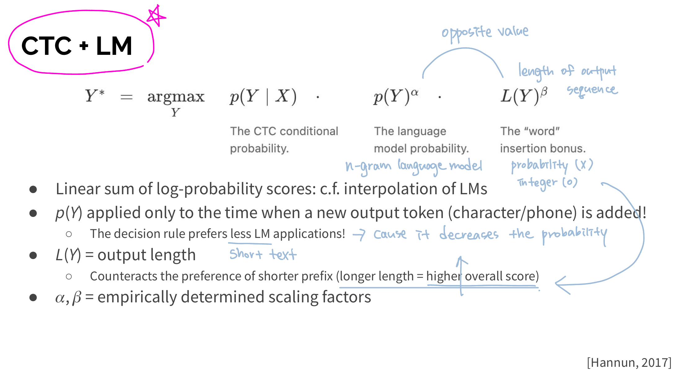
Shallow fusion is an inference-time technique that combines the scores from the acoustic model and an external language model in a linear interpolation. The core idea is to find the text sequence $\hat{y}$ that maximizes a combined score.

Since probabilities are often very small, it's standard practice to work with log-probabilities to maintain numerical stability. The combined score for a hypothesis $y$ given an audio input $x$ is calculated as follows:

Let's break this down.

• $\log P_{\text{AM}}(y|x)$: This is the acoustic model score. It's the log-probability of the hypothesis $y$ given the audio $x$, as calculated by the CTC model. This score comes directly from the neural network's outputs.

• $\log P_{\text{LM}}(y)$: This is the language model score. It's the log-probability of the hypothesis $y$ according to an external, pre-trained LM (like KenLM). This score reflects how grammatically and semantically likely the sentence is.

• $\lambda$ (lambda, often called lm_weight): This is the language model weight. It's a crucial hyperparameter that balances the influence of the AM and the LM.

  • If $\lambda$ is too low, the LM's contribution is negligible.
  • If $\lambda$ is too high, the system may output grammatically perfect but acoustically incorrect sentences, ignoring what was actually said.
  • Typical values are tuned on a validation set and often fall in the range of 0.5 to 2.0.

• $\beta \cdot \text{word\_count}(y)$: This is the word insertion bonus. CTC models have an inherent bias towards shorter sequences because they can merge repeated characters. This term adds a small bonus for each word in the hypothesis, counteracting the bias and preventing the decoder from favoring overly short (and often incorrect) transcriptions. $\beta$ is another hyperparameter to be tuned.

This entire calculation happens within the beam search algorithm at each step to score and prune candidate hypotheses.

4. Practical Implementation with torchaudio

Now let's see how this theoretical concept is put into practice. The torchaudio library provides a powerful and efficient CTC beam search decoder that has built-in support for shallow fusion with a KenLM language model.

Let's summarize the key steps from the torchaudio tutorial:

1. Gather Components: You need four things:

   • Acoustic Model: A trained CTC model, like wav2vec2.0-base-960h.
   • Tokens: A list of the possible characters the model can predict.
   • Lexicon: A mapping of words to their character sequences (e.g., HELLO H E L L O). This constrains the search to valid words.
   • Language Model: A KenLM n-gram model file (e.g., lm.bin). N-gram models are statistical (not neural), which makes them very fast and memory-efficient for inference.

2. Construct the Decoder: You instantiate the decoder using the torchaudio.models.decoder.ctc_decoder factory function, passing the paths to your tokens, lexicon, and LM files, along with the hyperparameters we discussed.

   from torchaudio.models.decoder import ctc_decoder
   
   beam_search_decoder = ctc_decoder(
       lexicon="path/to/lexicon.txt",
       tokens="path/to/tokens.txt",
       lm="path/to/lm.bin", # The Language Model
       nbest=1,
       beam_size=1500,
       lm_weight=1.8,      # This is our lambda (λ)
       word_score=-1.0,    # This contributes to our beta (β)
   )
   

3. Run Inference: You first get the emissions (log-probabilities) from your acoustic model for a given audio waveform. Then, you pass these emissions to the decoder object.

   
   
   
   # Assume `model` is your wav2vec 2.0 model and `waveform` is your audio
   with torch.no_grad():
       emissions, _ = model(waveform)
   
   
   
   
   # The decoder performs the shallow fusion beam search
   hypotheses = beam_search_decoder(emissions)
   
   
   
   
   # Print the best hypothesis
   print(hypotheses[0][0].words) 
   

As the tutorial demonstrates, the result from the beam search decoder with an LM is significantly more accurate and linguistically coherent than the output from a simple greedy decoder.

5. Shallow Fusion in Context

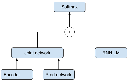
Shallow fusion is an effective and popular method, but it's not the only way to integrate an LM.

To summarize the trade-offs:

• Shallow Fusion:
  • Pros: Simple, flexible (you can swap LMs without retraining the AM), computationally cheap at training time (since it's an inference-only technique).
  • Cons: The AM is not aware of the LM during training, so the two models are not jointly optimized.
• Deep Fusion:
  • Pros: Potentially higher accuracy as the AM and LM are more tightly integrated during training.
  • Cons: More complex to implement, requires retraining the entire system, less flexible.

For many applications, the simplicity and effectiveness of shallow fusion make it an excellent choice.

Conclusion

In this lesson, we have demystified the process of integrating an external language model with a CTC-based acoustic model. You now understand not just why this is necessary but also how it works, from the high-level concept down to the mathematical formulation and practical code implementation.

Key Takeaways:

• Acoustic Models (AMs) predict what an audio signal sounds like, while Language Models (LMs) predict what sentences are linguistically probable.
• Shallow fusion combines the scores from a CTC-based AM and an external LM during beam search decoding to produce more accurate transcriptions.
• The core formula involves a weighted sum of log-probabilities: $\text{Score}=\log P_{\text{AM}}+\lambda \log P_{\text{LM}}+\text{bonus}$.
• Hyperparameters like the language model weight ($\lambda$) and a word insertion bonus ($\beta$) are critical for balancing the two models' influence.
• Libraries like torchaudio provide ready-to-use implementations of CTC beam search decoders with shallow fusion capabilities.

Preview of the Next Lesson:

We have now explored two dominant paradigms in ASR: the end-to-end encoder-decoder approach (Whisper) and the CTC-based approach augmented with shallow fusion (wav2vec 2.0). In our next lesson, we will directly "Compare the trade-offs between CTC, attention-based, and hybrid ASR systems." This will synthesize your knowledge and give you a framework for choosing the right architecture for a given ASR task.