Demystifying 70B Model Memory: VRAM & KV Cache

Introduction

Welcome back. In the last few lessons, you've built a solid foundation in LLM memory arithmetic. You've learned to calculate the VRAM required for the three primary consumers:

1. Model Weights: The static, core parameters of the model.
2. Activations: The temporary tensors created during the forward pass.
3. KV Cache: The dynamic storage for past keys and values, crucial for efficient autoregressive decoding.

Now, it's time to put it all together. This lesson synthesizes that knowledge to answer one of the core questions of this course: "Why is my 70B model using 120 GB of VRAM and still slow?"

Our learning outcome is to apply your VRAM and KV cache calculation skills to a 70-billion-parameter model to explain its large memory footprint. This exercise is not just theoretical; it's a "napkin math" simulation that every AI Systems Engineer must be able to perform for capacity planning, cost estimation, and performance debugging.

Breaking Down the Memory Footprint of a 70B Model

We will dissect the memory requirements of a canonical 70B model, like Llama 2 70B, piece by piece. This will give you a concrete mental model of where every gigabyte of VRAM goes.

1. The Foundation: Model Weights

The most straightforward component is the memory needed to simply load the model's parameters into the GPU. As you know, this is a function of the parameter count and the precision (the data type used to store each parameter).

As the article shows, the calculation is simple:

$$\text{Memory (GB)}=\frac{\text{Number of Parameters}\times \text{Bytes per Parameter}}{1024^3}$$

For a 70B model, this translates to:

• FP32 (4 bytes/param): 70B × 4 ≈ 280 GB
• FP16/BF16 (2 bytes/param): 70B × 2 = 140 GB
• INT8 (1 byte/param): 70B × 1 = 70 GB
• INT4 (0.5 bytes/param): 70B × 0.5 = 35 GB

Right away, you can see that even with half-precision (FP16/BF16), which is standard for inference, the weights alone require 140 GB, far exceeding the capacity of a single 80 GB H100 GPU. This is the first part of the answer to "Why so big?".

2. The Hidden Consumer: KV Cache

The model weights are static, but the KV cache is dynamic and can be just as memory-hungry. Its size depends not on the model's weight, but on its architecture and the runtime workload (batch size and sequence length).

Let's calculate the KV cache for a Llama 2 70B model. You'll need the formula from our last lesson and the model's specific architecture:

• Number of layers (L): 80
• Hidden dimension: 8,192
• Number of KV heads (H_kv): 8 (Llama 2 70B uses Grouped-Query Attention)
• Dimension per head (D_head): 128
• Precision (P): 2 bytes (for FP16)

The calculation shown in the article is:

$$\text{KV Cache (GB)}=\frac{2\times 8\times 4096\times 80\times 8\times 128\times 2}{1024^3}\approx 32\text{ GB}$$

(Batch Size = 8, Sequence Length = 4096)

This is a critical insight: for a batch of just 8 requests with a 4K context, the KV cache consumes an additional 32 GB. This is nearly the size of a 4-bit quantized 70B model!

The following graph vividly illustrates how this memory cost explodes with longer contexts.

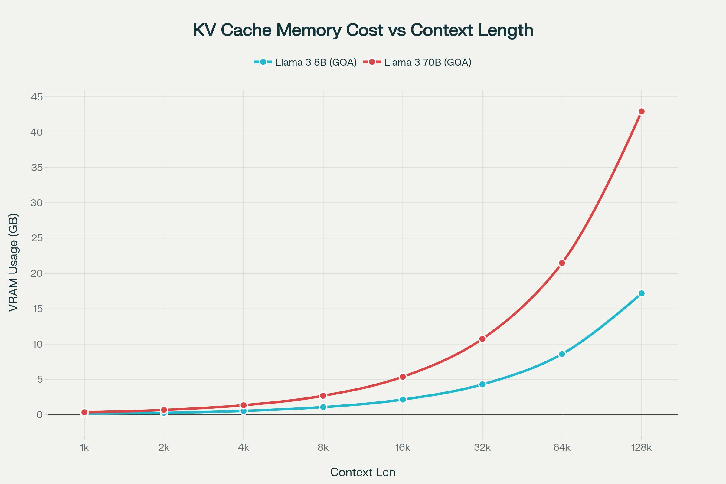
To really drive this point home, let's watch a short video that emphasizes the scale of KV cache consumption.

3. Putting It All Together: A Full VRAM Estimate

Now we can assemble the full picture. Total VRAM is not just weights and KV cache. We must also account for temporary activation memory and system overheads.

Let's review the final tally from the article for a Llama 2 70B model with a batch size of 16 and a 4K sequence length:

• Model Weights (FP16): 140 GB
• KV Cache: 64 GB (doubled from the previous example because batch size is now 16)
• Activations (Peak): ~24 GB (an approximation, but necessary to account for)
• System Overhead: ~8 GB (for PyTorch, CUDA kernels, etc.)
• Safety Buffer (10%): ~24 GB

Total Estimated VRAM: ~260 GB

This final number provides a clear, quantitative answer to our initial question. A 70B model requires hundreds of gigabytes of VRAM not just because of its 140 GB of weights, but because of the massive, dynamic KV cache needed to serve even a moderate number of users, plus additional overheads for computation and system software. This explains why you need a cluster of powerful GPUs (e.g., 4x H100 80GB) to serve such a model effectively.

Self-Check Exercise

Your turn to do the napkin math. Let's calculate the memory footprint for a different large model, Cohere's Command R+, which has 104 billion parameters.

Model: Command R+ (104B)

• Parameters: 104B
• Number of layers (L): 64
• Number of KV heads (H_kv): 96 (It uses Multi-Head Attention, so num_kv_heads = num_attention_heads)
• Dimension per head (D_head): 128

Scenario:

• Batch Size (B): 8
• Max Sequence Length (S): 8192
• Precision (P): bfloat16 (2 bytes)

Calculate the following:

1. VRAM for model weights.
2. VRAM for the KV cache.
3. A total VRAM estimate, assuming ~15 GB for activations and system overhead combined.

View Solution

1. Model Weights Memory:

$$\text{Weights (GB)}=\frac{104\times 10^9\times 2}{1024^3}\approx 193.7\text{ GB}$$

Just loading the model in bf16 requires nearly 200 GB of VRAM.

2. KV Cache Memory:
Using the formula 2 * B * S * L * H_kv * D_head * P:

$$\text{KV Cache (Bytes)}=2\times 8\times 8192\times 64\times 96\times 128\times 2=206,158,430,208\text{ bytes}$$ $$\text{KV Cache (GB)}=\frac{206,158,430,208}{1024^3}\approx 192.0\text{ GB}$$

For a batch of 8 requests with an 8K context, the KV cache is almost as large as the model weights themselves!

3. Total Estimated VRAM:

$$\text{Total VRAM}=\text{Weights}+\text{KV Cache}+\text{Overheads}$$ $$\text{Total VRAM}\approx 193.7\text{ GB}+192.0\text{ GB}+15\text{ GB}\approx 400.7\text{ GB}$$

To serve this workload, you would need at least 401 GB of VRAM, which could be provisioned with a cluster of 8x H100 80GB GPUs (640 GB total capacity), giving you headroom.

Conclusion

In this lesson, you synthesized your knowledge of memory arithmetic to create a complete VRAM budget for a 70B model.

Key Takeaways:

• A large model's memory footprint is a sum of multiple components: Model Weights, KV Cache, Activations, and System Overheads.
• For a 70B model, the weights alone (at 140 GB in FP16) require a multi-GPU setup.
• The KV cache is a massive, dynamic consumer of VRAM that scales with batch size and sequence length. In many production scenarios, its size can equal or even exceed the memory required for the model weights.
• This "napkin math" is a fundamental skill for designing, provisioning, and debugging LLM serving systems, allowing you to make informed decisions about hardware, batching strategies, and context length limits.

You have now completed the module on LLM internals and memory arithmetic. You have the full request-to-token mental model and can precisely account for where memory goes.

Preview of the Next Module:

Memory is only one half of the equation. The other is compute. In our next module, Compute Optimization, we will begin by analyzing the computational characteristics of a transformer. You will learn to distinguish between compute-bound and memory-bandwidth-bound operations, a critical step in understanding why an LLM can be slow and how to make it faster.