Word2Vec with Negative Sampling

Hello! Welcome to the first lesson of our new module, "Foundations of Language Modeling and Embeddings."

In the previous module, we meticulously constructed a complete Transformer architecture. We saw how it processes sequences of numerical vectors to perform complex tasks like machine translation. But this raises a fundamental question: how do we get those meaningful numerical vectors from raw text in the first place? This module will answer that question, starting with one of the most foundational techniques.

Today, your learning outcome is to train word embeddings using the Word2Vec (Skip-gram) model with negative sampling. We will explore how we can learn dense vector representations of words that capture their semantic meanings, based on the contexts in which they appear.

By the end of this lesson, you will understand:

• Why simple numerical representations like one-hot encoding are insufficient for language tasks.
• The core intuition behind Word2Vec and its two main architectures: Skip-gram and CBOW.
• The architecture of the Skip-gram model and how it uses a neural network to learn embeddings.
• The computational challenge of the standard softmax output and how negative sampling provides an elegant and efficient solution.
• How to implement and train a Skip-gram model with negative sampling from scratch using PyTorch.

1. The Need for Word Embeddings

Machine learning models, including the Transformer we just built, are mathematical functions. They operate on numbers, not on abstract symbols like words. Therefore, our first challenge in any Natural Language Processing (NLP) task is to convert words into a numerical format.

A naive approach is one-hot encoding, where each word in our vocabulary is represented by a long vector filled with zeros, except for a single '1' at the index corresponding to that word.

# Vocabulary: [the, quick, brown, fox, jumps]
the   = [1, 0, 0, 0, 0]
quick = [0, 1, 0, 0, 0]
brown = [0, 0, 1, 0, 0]
...

While simple, this method has critical flaws:

1. Sparsity & Inefficiency: For a realistic vocabulary of 50,000 words, each word vector would have 50,000 dimensions, wasting memory and computational resources.
2. Lack of Semantic Relationship: The one-hot vectors for "king" and "queen" are mathematically as different from each other as the vectors for "king" and "apple". The dot product between any two distinct word vectors is zero, implying they are all orthogonal and unrelated.

We need a better way. We want dense, lower-dimensional vectors (called embeddings) where similar words have similar vector representations. This is the core idea behind word embeddings.

2. Word2Vec: Learning Embeddings from Context

In 2013, researchers at Google led by Tomas Mikolov introduced Word2Vec, a landmark technique for learning word embeddings. Its guiding principle is the distributional hypothesis, famously summarized by linguist John Rupert Firth: "You shall know a word by the company it keeps."

In other words, words that frequently appear in similar contexts tend to have similar meanings. Word2Vec formalizes this idea by training a shallow neural network on a predictive task. There are two primary architectures:

1. Continuous Bag-of-Words (CBOW): The model predicts a target (center) word based on its surrounding context words.
2. Skip-gram: The model does the reverse. It predicts the surrounding context words given a single center word.

While both are effective, Skip-gram is known to perform better with large datasets and is particularly good at learning representations for rare words. For this reason, we will focus on the Skip-gram architecture.

3. The Skip-gram Architecture (Naive Approach)

The goal of Skip-gram is to learn word vector representations that are good at predicting nearby words. Let's take the sentence "The quick brown fox jumps over the lazy dog." If our center word is "fox" and we use a window_size of 2, the context words are "quick", "brown", "jumps", and "over". The model's task is to predict these context words given "fox".

This is framed as a supervised learning problem and solved with a simple neural network.

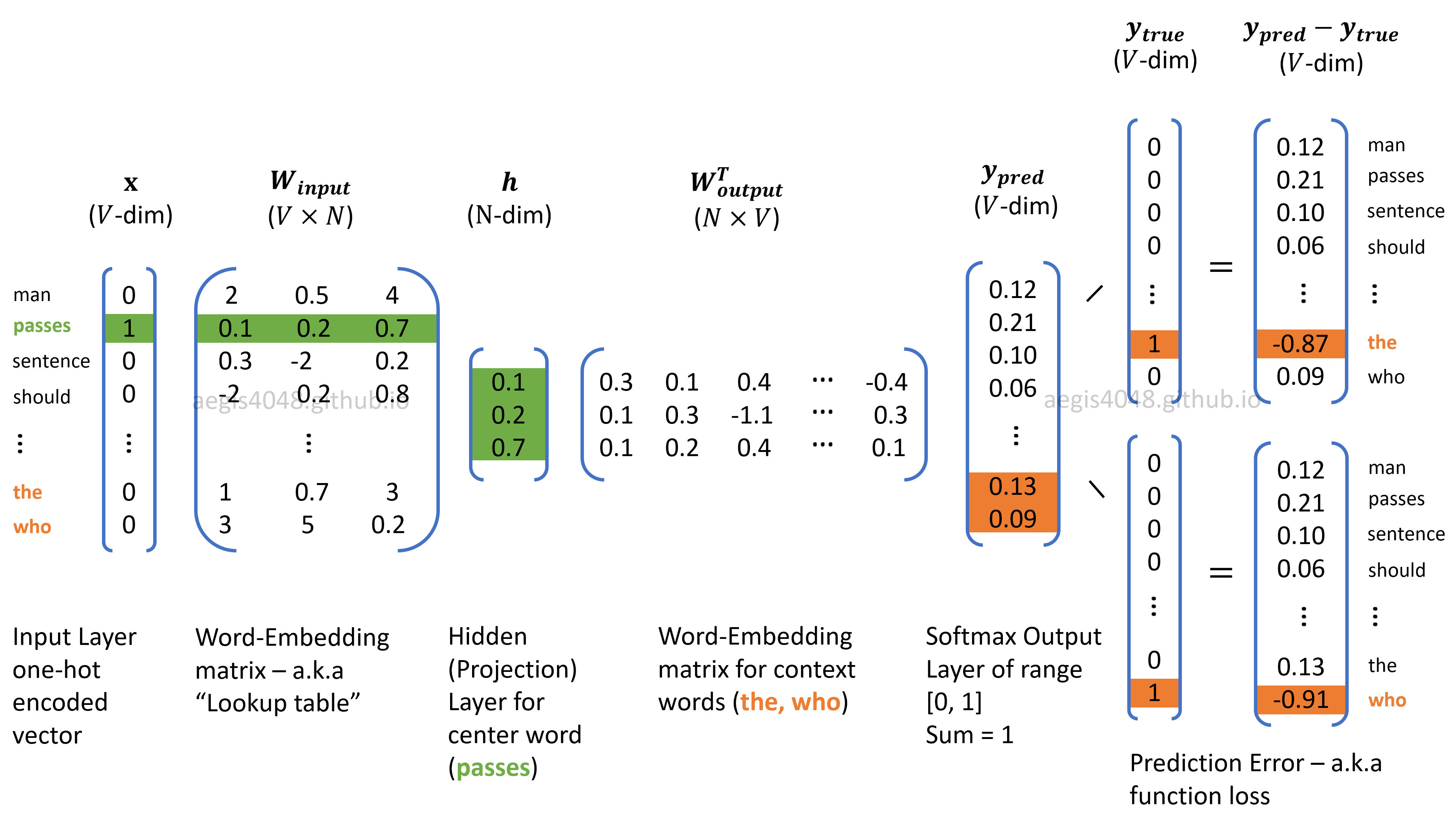
Let's break down this architecture:

1. Input Layer: A one-hot encoded vector representing the center word (e.g., "fox"). Its dimension is V, the size of our vocabulary.
2. Input Embedding Matrix W_input: A weight matrix of size V x N, where N is the desired embedding dimension (e.g., 300). Multiplying the one-hot input vector by this matrix is equivalent to simply looking up the row corresponding to the input word. This row vector is the word's embedding.
3. Hidden/Projection Layer: This layer is just the 1 x N vector looked up from W_input. There's no activation function here.
4. Output Embedding Matrix W_output: Another weight matrix, this time of size N x V.
5. Output Layer: The hidden layer vector is multiplied by W_output, resulting in a 1 x V vector. This vector contains a score for every word in the vocabulary, indicating how likely it is to be a context word.
6. Softmax Activation: A softmax function is applied to the output layer scores to turn them into a probability distribution. We want the probabilities for the true context words (e.g., "quick", "brown") to be high, and low for all other words.

The model is trained by adjusting the weights in W_input and W_output to minimize the prediction error (e.g., using cross-entropy loss). After training, we typically discard W_output and use the learned W_input matrix as our final word embeddings.

The Computational Bottleneck

This approach seems straightforward, but there's a huge problem. Look at the softmax function in the output layer. For every single training example, calculating the normalization term in the denominator requires summing over all V words in the vocabulary.

$$P(w_{context}|w_{center})=\frac{\exp (v_{w_{context}}^{\prime }\cdot v_{w_{center}})}{{\sum }_{i=1}^V\exp (v_{w_i}^{\prime }\cdot v_{w_{center}})}$$

If our vocabulary has a million words (V = 1,000,000), this calculation is extremely expensive and makes training prohibitively slow. The algorithm's complexity is O(V). We need a more efficient way to train.

4. The Solution: Negative Sampling

Instead of a massive multi-class classification problem, negative sampling reframes the task into a series of much simpler binary classification problems.

The new question is: Given a pair of words (center_word, context_word), is it a "real" pair from our text (a positive sample), or is it a "fake" pair where the context word was randomly drawn from the vocabulary (a negative sample)?

Here's how it works for a single (center, context) pair:

1. Treat the actual pair (e.g., "fox", "jumps") as a positive sample. The model should be trained to output a high probability (close to 1) for this pair.
2. Create k negative samples by pairing the same center word with k randomly chosen words from the vocabulary (e.g., "fox", "chair"; "fox", "galaxy"). These are words that did not appear in the context. The model should be trained to output a low probability (close to 0) for these pairs.
3. The neural network now only needs to compute the scores for k+1 words (1 positive, k negative) instead of all V words. A sigmoid function is used on each output score to get the binary probability.
4. The loss is then the sum of the binary cross-entropy losses for these k+1 classification tasks.

This change reduces the complexity from O(V) to O(k+1). Since k is typically small (5-20), the training speedup is immense.

5. Training with PyTorch: A Practical Implementation

Now, let's bring theory into practice. Given your software engineering background, the most effective way to solidify your understanding is to see how this is implemented in code. We'll use PyTorch to build and train a Skip-gram model with negative sampling.

The core of the model will consist of two nn.Embedding layers: one for the target (center) words and one for the context words.

import torch.nn as nn

class SkipGramNegativeSampling(nn.Module):
    def __init__(self, vocab_size, embed_dim):
        super(SkipGramNegativeSampling, self).__init__()
        # Embeddings for center words
        self.target_embed = nn.Embedding(vocab_size, embed_dim)
        # Embeddings for context words
        self.context_embed = nn.Embedding(vocab_size, embed_dim)
        # Initialize weights
        self.target_embed.weight.data.uniform_(-1, 1)
        self.context_embed.weight.data.uniform_(-1, 1)

    def forward(self, target, context):
        # target: (batch_size)
        # context: (batch_size, num_samples) where num_samples = 1 (positive) + k (negative)
        
        # Get embeddings
        u = self.target_embed(target) # (batch_size, embed_dim)
        v = self.context_embed(context) # (batch_size, num_samples, embed_dim)
        
        # Reshape u for dot product
        u = u.unsqueeze(2) # (batch_size, embed_dim, 1)
        
        # Dot product
        logits = torch.bmm(v, u).squeeze() # (batch_size, num_samples)
        
        return logits

The training process involves feeding positive and negative pairs to this model and calculating a binary cross-entropy loss.

Test your understanding!

You are training a Word2Vec Skip-gram model with negative sampling.

• Vocabulary size V = 10000
• Embedding dimension N = 100
• Number of negative samples k = 5

1. What are the dimensions of the two embedding matrices (W_input and W_output) in your model?
2. For a single training pair (center_word, positive_context_word), how many forward passes (or dot products) does the model compute to calculate the loss?
3. Why is BCEWithLogitsLoss a suitable loss function for this task, as opposed to CrossEntropyLoss which we might have used with the softmax approach?

Show answer

1. Both embedding matrices, W_input (for target/center words) and W_output (for context words), will have the dimensions V x N, which is 10000 x 100.
2. The model computes k + 1 dot products. It calculates the dot product of the center word's embedding with the positive context word's embedding, and also with the k=5 negative samples' embeddings. So, a total of 6 dot products are computed.
3. BCEWithLogitsLoss (Binary Cross-Entropy Loss) is suitable because negative sampling turns the problem into a set of independent binary classification tasks. For each pair (positive or negative), the model predicts a single score (logit) and we want to classify it as either correct (1) or incorrect (0). CrossEntropyLoss is designed for multi-class classification where the classes are mutually exclusive (i.e., predicting one correct class out of many), which is the setup for the original softmax approach, not for negative sampling.

Conclusion

In this lesson, we have taken a crucial first step into the world of language representation. You've learned how to move beyond simple, inefficient encodings to create rich, meaningful word embeddings that capture semantic relationships.

Key Takeaways:

• Word embeddings are dense vector representations that capture the meaning of words based on their usage.
• The Word2Vec Skip-gram model trains a neural network to predict context words from a center word.
• The standard softmax output is computationally too expensive for large vocabularies.
• Negative sampling provides a highly efficient alternative by reframing the task as a series of binary classifications (positive vs. negative samples).
• The core of the implementation involves two embedding matrices and a training loop that optimizes a binary cross-entropy loss.

After training, these embeddings can be used for various tasks, such as finding word similarities (vector('king') - vector('man') + vector('woman') results in a vector very close to vector('queen')) or as the initial input layer for more complex models like LSTMs or Transformers.

Preview of the Next Lesson:
While Word2Vec operates on whole words, modern NLP systems often need to handle sub-word units to deal with rare words, typos, and rich morphologies. In our next lesson, we will explore advanced tokenization techniques, including Byte-Pair Encoding (BPE), which is fundamental to how models like GPT and BERT process text.