Deep Learning for Text-to-Speech Synthesis

Hello! Welcome to our next lesson on Multimodal AI.

In our last session, we explored how the Whisper model masterfully converts human speech into text (ASR). We saw how it uses a Transformer encoder-decoder architecture to process log-Mel spectrograms and generate accurate transcriptions.

Today, we will tackle the inverse problem, fulfilling the learning outcome: Build a text-to-speech (TTS) system using a deep learning approach. We'll journey from text input to a synthesized audio waveform, deconstructing the elegant architectures that make machines speak. You'll understand the components of a modern TTS pipeline, dissect a key model architecture, and learn how to both use pre-trained systems and train your own.

1. The Modern Deep Learning TTS Pipeline

Just as ASR isn't a single step, modern TTS is a multi-stage process. While ASR goes Waveform -> Spectrogram -> Text, TTS essentially reverses this flow. Let's get a high-level overview of the components that form a typical deep learning TTS system.

As the video outlines, a typical deep learning TTS pipeline consists of two main models, preceded by a text-processing step:

1. Text Frontend (Text Normalization & Phonemization): Raw text is messy. It contains numbers ("1984"), abbreviations ("Dr."), and punctuation. The first step is to clean this text and convert it into a phonetic representation. For example, "The cat sat." becomes something like [DH, AH, K, AE, T, S, AE, T, .]. This is done using a Grapheme-to-Phoneme (G2P) converter. This gives the model a consistent, unambiguous representation of the sounds to produce.

2. Acoustic Model (e.g., FastSpeech 2, Tacotron 2): This is the heart of the system. It takes the sequence of phonemes and generates a log-Mel spectrogram. This is the exact same kind of spectrogram we saw Whisper use as its input. The acoustic model's job is to predict the spectral content of the speech over time, effectively translating the symbolic phonemes into a detailed acoustic plan.

3. Vocoder (e.g., HiFi-GAN, WaveNet): A spectrogram is a visual representation of sound, not sound itself. The vocoder is a separate neural network that takes the spectrogram from the acoustic model and synthesizes the final audio waveform. Its job is to "invert" the spectrogram, filling in the phase information and other details needed to create a high-fidelity, audible sound wave.

This two-stage approach (Acoustic Model + Vocoder) is a very common and successful paradigm in TTS.

2. A Deep Dive into the Acoustic Model: FastSpeech 2

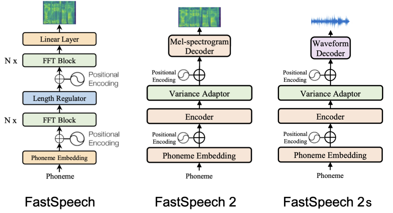
The most interesting architectural innovations often happen in the acoustic model. Let's dissect FastSpeech 2, a highly influential non-autoregressive model that addresses many challenges in TTS.

Unlike autoregressive models (like the Whisper decoder) that generate output one step at a time, FastSpeech 2 generates the entire spectrogram in parallel. This makes it extremely fast for inference.

Let's look at its architecture.

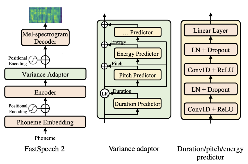
This architecture can be broken down into four key parts:

1. Phoneme Encoder: A standard Transformer encoder (using feed-forward networks and self-attention, which you're familiar with) processes the input phoneme sequence. It produces a sequence of hidden states, one for each phoneme, that are contextually aware.

2. Variance Adaptor: This is the core innovation of FastSpeech 2. The phoneme sequence is a very sparse representation. It doesn't tell the model how long to hold each sound, at what pitch to say it, or with what energy. The Variance Adaptor injects this crucial prosodic information.

   • Duration Predictor: It predicts the duration (in spectrogram frames) for each phoneme. This is critical for non-autoregressive models, as it solves the alignment problem: how to expand the phoneme sequence to match the length of the audio.
   • Pitch Predictor: It predicts the fundamental frequency (pitch contour) for each phoneme.
   • Energy Predictor: It predicts the average energy (related to loudness) of each phoneme.

3. Length Regulator: Using the predicted durations, this simple module expands the encoder's hidden states. For example, if the phoneme /k/ has a predicted duration of 4, the Length Regulator repeats the hidden state for /k/ four times.

4. Mel-Spectrogram Decoder: Another Transformer-style decoder takes the expanded and prosody-enriched sequence and generates the final mel-spectrogram.

The diagram below gives a comparative view, showing how FastSpeech 2 improves upon the original FastSpeech.

Test your understanding!

In our last lesson, the Whisper decoder used autoregressive generation. FastSpeech 2 is non-autoregressive. What component of the FastSpeech 2 architecture is the key enabler for this parallel, non-autoregressive generation, and why?

Show answer

The Duration Predictor (within the Variance Adaptor) is the key. In an autoregressive model, the decision to stop generating frames for one sound and start the next is learned implicitly. The model just keeps generating until it predicts an "end" token or a new phoneme. In a non-autoregressive model, you need to know the full length of the output in advance. The Duration Predictor explicitly provides this information, allowing the model to allocate the correct number of frames for each phoneme and generate the entire spectrogram in one go.

3. Practical Application: From Theory to Code

Now that we understand the components, let's see how to build a TTS system in practice. We'll explore two approaches: using pre-trained models for immediate results, and training a model on custom voice data.

Approach 1: Assembling a Pre-trained System

Libraries like SpeechBrain and Hugging Face Transformers provide pre-trained models that we can easily assemble. The following example uses SpeechBrain to implement the two-stage pipeline we just discussed, combining a FastSpeech2 acoustic model with a HiFiGAN vocoder.

Here's the core logic from that resource, which you can run in a Python environment:

# You may need to install SpeechBrain first: pip install speechbrain
import torchaudio
from speechbrain.inference.TTS import FastSpeech2
from speechbrain.inference.vocoders import HIFIGAN

# 1. Load the two main components: Acoustic Model and Vocoder
fastspeech2 = FastSpeech2.from_hparams(source="speechbrain/tts-fastspeech2-ljspeech")
hifi_gan = HIFIGAN.from_hparams(source="speechbrain/tts-hifigan-ljspeech")

# Input text
input_text = "Hello, this is a test of a text to speech system."

# 2. Run the Acoustic Model (text -> spectrogram)
# This also returns predicted durations, pitch, and energy
mel_output, durations, pitch, energy = fastspeech2.encode_text([input_text])

# 3. Run the Vocoder (spectrogram -> waveform)
waveforms = hifi_gan.decode_batch(mel_output)

# 4. Save the final audio
torchaudio.save('example_tts.wav', waveforms.squeeze(1), 22050)

print("TTS audio saved to example_tts.wav")

More recent models, like VITS (Variational Inference with adversarial learning for end-to-end Text-to-Speech), integrate the acoustic model and vocoder into a single end-to-end network. This simplifies the inference process, as you only need to interact with one model.

Using the Hugging Face pipeline, generating speech with VITS is even more straightforward:

# You will need transformers, torch, and scipy: pip install transformers torch scipy
from transformers import pipeline
from scipy.io.wavfile import write

# The pipeline handles loading the model and all pre/post-processing
synthesiser = pipeline("text-to-speech", "facebook/mms-tts-eng")

speech = synthesiser("Hello, this is a test of an end-to-end speech system.")

# The pipeline output is a dictionary containing the audio and sampling rate
write("example_vits.wav", rate=speech["sampling_rate"], data=speech["audio"])

print("TTS audio saved to example_vits.wav")

Approach 2: Training a Custom Voice Model (Voice Cloning)

What if you want the TTS system to speak in a specific voice, maybe even your own? This is known as voice cloning, and it involves training a TTS model on a custom dataset. This is the ultimate way to "build a TTS system."

The process is a classic supervised machine learning workflow:

1. Data Collection: Record short audio clips of the target voice.
2. Data Preparation: Transcribe each audio clip precisely. You need to create a manifest file (like a CSV or text file) that maps each audio file to its exact text content.
3. Preprocessing: Ensure all audio files have the same format (e.g., sample rate, bit depth, single channel/mono).
4. Training: Fine-tune a pre-trained TTS model (like Tacotron 2 or FastSpeech 2) on your custom audio-text pairs.
5. Inference: Use the newly trained model to synthesize speech in the target voice.

The video makes a crucial point: the quality and naturalness of the synthesized voice are directly proportional to the amount and quality of the training data. A model trained on just 25 short clips will sound robotic and garbled, while one trained on hours of clean audio can be remarkably realistic.

Conclusion

In this lesson, you've completed the other half of the speech AI equation. We've gone from text to a rich acoustic plan (spectrogram) and finally to an audible waveform.

Key Takeaways:

• Deep learning TTS systems typically use a two-stage pipeline: an Acoustic Model (text-to-spectrogram) and a Vocoder (spectrogram-to-waveform).
• Models like FastSpeech 2 use a non-autoregressive Transformer architecture with a Variance Adaptor to predict and control prosodic elements like duration, pitch, and energy, enabling fast and high-quality synthesis.
• More modern architectures like VITS offer an end-to-end solution, simplifying the pipeline by integrating the acoustic model and vocoder.
• "Building" a TTS system can mean either assembling pre-trained components for inference or undergoing the full supervised learning process of collecting, preparing, and training on a custom audio-text dataset to clone a specific voice.
• For custom training, the quantity and quality of the dataset are the most critical factors determining the final output quality.

Preview of the Next Lesson:

We've now covered foundational models for understanding and generating both text and speech. In the next module, "Specialized Generative Applications," we will push these concepts further. Our first lesson will be to Fine-tune a language model for NSFW or uncensored text generation. This will take us from the public-facing, general-purpose models we've studied into the world of model specialization and the techniques used to adapt them for specific, and sometimes controversial, domains, directly addressing an interest you expressed.