Spectrogram Generation for Deep Learning

Hello! Welcome to the next lesson in our journey through Multimodal and Cross-Domain AI.

In our previous lesson, we built a Visual Question Answering (VQA) model, diving deep into how to fuse visual and textual information to answer specific queries about an image. We've now established a strong foundation in combining vision and language. Today, we pivot to a new and fascinating modality: audio.

This lesson addresses the learning outcome: Process audio signals into spectrograms for deep learning models. We'll explore how to transform a one-dimensional audio waveform into a two-dimensional, image-like representation that is perfect for the deep learning architectures you're already familiar with, such as CNNs and Transformers. This transformation is the critical first step for almost any modern audio-related AI task, from speech recognition to music classification.

1. From Sound Wave to Frequency Spectrum

At its core, a digital audio signal is a simple time series: a long sequence of numbers representing the amplitude of a sound wave at discrete points in time. This is the time-domain representation.

While a raw waveform contains all the information, it's not in a format that's easy for neural networks to learn from. The key acoustic features, like pitch and timbre, are encoded in the signal's frequencies, not directly in its amplitude over time.

The Fourier Transform (FT) is the mathematical tool that decomposes a signal into its constituent frequencies, moving us from the time domain to the frequency domain. However, a standard FT applied to an entire audio clip tells you what frequencies were present, but loses all information about when they occurred. For speech or music, timing is everything.

2. The Spectrogram: Capturing Time and Frequency

To solve this, we use the Short-Time Fourier Transform (STFT). The idea is wonderfully simple:

1. Divide the long audio signal into many small, overlapping time windows.
2. Apply the Fast Fourier Transform (FFT), an efficient algorithm for computing the FT, to each individual window.
3. Stack these FFT results side-by-side.

The result is a spectrogram: a 2D representation where the x-axis is time, the y-axis is frequency, and the color intensity at each point represents the amplitude (or energy) of a specific frequency at a specific time. It’s essentially an "image of sound."

Now, let's dive a bit deeper into the mechanics of STFT and how we derive the power spectrum.

We now have a standard spectrogram. For many scientific signals, this would be sufficient. But for audio meant for human ears, there's a crucial missing piece.

3. The Perception Problem: Linear vs. Logarithmic Hearing

A standard spectrogram's frequency axis is linear, measured in Hertz (Hz). This means the distance between 100 Hz and 200 Hz is treated the same as the distance between 10,000 Hz and 10,100 Hz.

However, human hearing doesn't work this way. We perceive pitch on a logarithmic scale. We are very sensitive to changes in low frequencies but much less so to equivalent changes in high frequencies.

To create a feature representation that is useful for tasks involving human speech or music, we need a frequency scale that mirrors our perception.

4. The Solution: Mel Spectrograms

This brings us to the Mel scale, a perceptual scale of pitches judged by listeners to be equal in distance from one another. The name "Mel" comes from "melody," highlighting its connection to pitch perception. By converting frequencies from Hertz to the Mel scale, we create a representation that is more aligned with how humans hear.

A Mel spectrogram is a spectrogram where the frequency axis is converted to the Mel scale. This process involves a fascinating piece of signal processing: the Mel filter bank.

Building the Mel Spectrogram

The process can be summarized in three steps:

1. Compute a standard power spectrogram using STFT.
2. Create a Mel filter bank, which is a set of triangular filters. These filters are narrow and closely spaced at low frequencies and become wider and more spread out at high frequencies, mimicking the logarithmic nature of human hearing.
3. Apply this filter bank to the spectrogram. Each filter collects the energy from its corresponding frequency band, effectively warping the spectrogram's frequency axis onto the Mel scale.

This "application" is a matrix multiplication, an efficient operation you are very familiar with. The Mel filter bank is a matrix that, when multiplied with the spectrogram matrix, transforms the frequency bins. The final common step is to take the logarithm of the resulting amplitudes, converting them to decibels (dB). This is also perceptually motivated, as we perceive loudness logarithmically. The final result is often called a log-Mel spectrogram.

Test your understanding!

A machine learning model is being designed for two different audio tasks:

1. Analyzing the high-frequency vibrations of a jet engine for predictive maintenance.
2. Transcribing human speech into text.

For which task would a Mel spectrogram be more suitable, and why? For the other task, what might be a better choice?

Show answer

A Mel spectrogram would be far more suitable for the speech transcription task. The Mel scale is designed to mimic human auditory perception, which emphasizes resolution in lower frequencies where most of the rich information in speech (like vowels and formants) resides.

For analyzing jet engine vibrations, a standard linear spectrogram would likely be more appropriate. The machine's frequencies of interest might be distributed linearly, and there's no reason to believe that a human perceptual scale would be relevant. Using a Mel spectrogram could risk compressing and losing important information in the high-frequency ranges.

5. The Final Product

After this entire process, we have our final representation: a log-Mel spectrogram. It has all the desirable properties for a deep learning model.

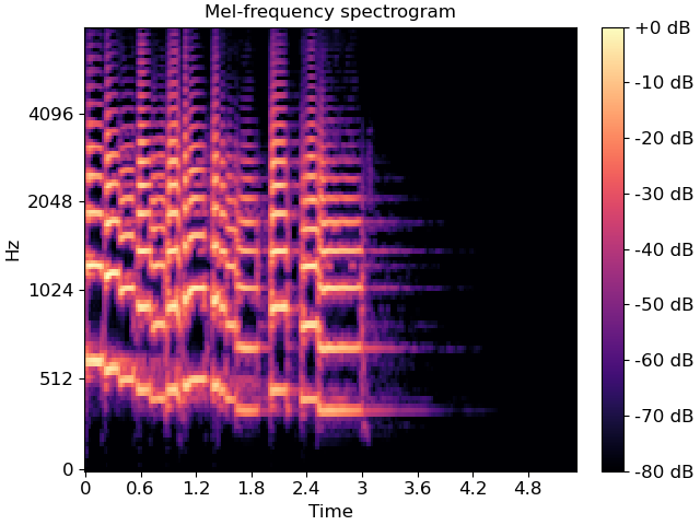
This 2D representation can now be treated just like an image. You can feed it into a CNN to learn local spatio-temporal features, or into a Vision Transformer (with patches taken from the spectrogram) to capture global relationships, effectively leveraging the powerful computer vision models we've already studied.

In practice, you won't need to implement this from scratch. Libraries like librosa in Python make it straightforward. A single function call can perform this entire complex pipeline:

import librosa
import librosa.display
import matplotlib.pyplot as plt
import numpy as np

# Load an example audio file
y, sr = librosa.load(librosa.ex('trumpet'))

# Compute the Mel spectrogram
M = librosa.feature.melspectrogram(y=y, sr=sr)

# Convert to decibels (log scale)
M_db = librosa.power_to_db(M, ref=np.max)

# Display the spectrogram
fig, ax = plt.subplots()
img = librosa.display.specshow(M_db, x_axis='time', y_axis='mel', sr=sr, ax=ax)
fig.colorbar(img, ax=ax, format='%+2.0f dB')
ax.set(title='Mel-frequency spectrogram')
plt.show()

Conclusion

In this lesson, we have built the bridge from raw, one-dimensional audio signals to rich, two-dimensional representations ready for deep learning. You've learned not just how to create these representations, but why each step is crucial.

Key Takeaways:

• Raw audio is a time-domain signal that is difficult for neural networks to interpret directly.
• The Short-Time Fourier Transform (STFT) converts an audio signal into a spectrogram, a 2D representation of frequency over time.
• Standard spectrograms use a linear frequency scale (Hertz), which does not match human auditory perception.
• The Mel scale is a perceptual scale that is logarithmic in nature, providing more resolution at lower frequencies.
• A Mel spectrogram is created by applying a Mel filter bank to a standard spectrogram, warping the frequency axis to the Mel scale. This is typically done via efficient matrix multiplication.
• The resulting log-Mel spectrogram is an image-like representation of sound, making it a perfect input for modern deep learning models like CNNs and Transformers.

Preview of the Next Lesson:

Now that you have mastered the art of creating the ideal audio representation, we will put it to use. In our next lesson, we will apply the Whisper architecture for robust automatic speech recognition (ASR). You will see how the Mel spectrograms we've just created serve as the direct input to this state-of-the-art model, enabling it to transcribe speech with remarkable accuracy.