Configure Authenticated FlyWire Notebook and Record Query Metadata

Welcome to the programmatic-analysis portion of the course. The next modules will use FlyWire data in Python, but reliable analysis starts with a small discipline: every query must be tied to a particular dataset, materialized snapshot, and coordinate convention. Otherwise, a notebook may run successfully while referring to a different reconstruction state from the one you intended.

By the end of this lesson, you will have a local Jupyter notebook that authenticates to FlyWire’s CAVE services, explicitly targets the public FlyWire dataset, discovers an available materialization at runtime, and writes a compact provenance record for later neuron and synapse queries.

---

Why configuration is scientific provenance, not boilerplate

A FlyWire neuron identifier is not permanently fixed. Proofreading can merge or split reconstruction fragments, which can change the root ID representing a neuron. Meanwhile, annotations and synapses are associated with physical locations in the EM volume. CAVE periodically resolves those locations against the current segmentation and stores versioned table snapshots called materializations.

For every later analysis, record these four items:

Item	What it fixes	Why it matters
Dataset / release	Public, Production, or Sandbox data	These serve different purposes and have different access rules.
Datastack	A specific imagery-and-segmentation collection	This is the target used by CAVEclient.
Materialization version	A snapshot of tables such as synapses and annotations	It makes query results reproducible despite later proofreading.
Coordinate convention	Axis order, physical units, and voxel resolution	It prevents querying the wrong location or mixing UI/API coordinates.

For this course, begin with the Public dataset. It is the appropriate default for reproducible learning and analysis. Do not switch a notebook to Production merely because it is newer: Production reflects live community proofreading and requires separate approval. Sandbox is useful for interface practice, but it is not the dataset to use for a stable connectomics result.

A useful mental model is:

• Segmentation is the current interpretation of which image voxels belong together.
• Root IDs name connected reconstructed objects in that segmentation.
• Materializations are dated, query-efficient snapshots that connect spatial annotations and synaptic locations to root IDs.
• Your notebook provenance states precisely which interpretation you analyzed.

---

Create a safe local authentication setup

Use a dedicated notebook, for example:

00_environment_and_provenance.ipynb

Install the two packages in the same Python environment as Jupyter. Run this cell once, then restart the kernel if Jupyter reports that a newly installed package cannot be imported.

%pip install -U caveclient fafbseg pandas

CAVE authentication uses a token. Obtain the token through the FlyWire/CAVE authentication workflow associated with your account, but do not paste it into a notebook, commit it to Git, or include it in a shared notebook export.

Instead, set it in the environment before launching Jupyter.

macOS/Linux shell:

export CAVE_TOKEN="paste-your-token-here"
jupyter lab

PowerShell:

$env:CAVE_TOKEN = "paste-your-token-here"
jupyter lab

The token is then available only to processes launched from that shell session. In a more durable local setup, use your operating system’s secret store or a local, ignored environment file; the essential point is that the secret remains outside version-controlled code.

Now create the first notebook cell:

import os
from datetime import datetime, timezone
from importlib.metadata import version

import pandas as pd
from caveclient import CAVEclient
from fafbseg import flywire

token = os.getenv("CAVE_TOKEN")

if not token:
    raise RuntimeError(
        "CAVE_TOKEN is not set. Set it in your shell, then restart Jupyter from that shell."
    )

# Store the token in CAVEclient's local credential mechanism.
bootstrap_client = CAVEclient()
bootstrap_client.auth.save_token(token)

print("Authentication token saved locally for CAVEclient.")
print("caveclient:", version("caveclient"))
print("fafbseg:", version("fafbseg"))

The token is not printed. That is intentional.

---

Pin the FlyWire dataset and datastack

Set these values explicitly near the top of every analysis notebook. Avoid relying on a package default, because an unnoticed default change can alter later results.

DATASET = "public"
DATASTACK = "flywire_fafb_public"

flywire.set_default_dataset(DATASET)

client = CAVEclient(datastack_name=DATASTACK)

available_datastacks = bootstrap_client.info.get_datastacks()

if DATASTACK not in available_datastacks:
    raise RuntimeError(
        f"{DATASTACK!r} was not returned by the service. "
        "Check your network connection, token, and current FlyWire documentation."
    )

datastack_info = client.info.get_datastack_info()

print("Dataset:", DATASET)
print("Datastack:", DATASTACK)
print("Datastack metadata retrieved successfully.")

This is your first operational test:

1. bootstrap_client verifies that the token can access global CAVE services.
2. client is bound to the intended FlyWire datastack.
3. get_datastack_info() verifies that the chosen datastack is available to your account.

A successful result does not establish that a particular neuron ID is valid. That will be the subject of the next lesson. It only establishes a correctly authenticated and targeted analysis environment.

A datastack is more precise than a project nickname. It identifies a coordinated collection of imagery and segmentation data. Record it even when its name appears obvious from the notebook title.

---

Select and record one materialization

Ask FlyWire which materializations are available now. Do not copy the version number from an old tutorial: documentation examples reflect the versions available when they were written, while your code should record the versions available when you ran it.

materializations = flywire.get_materialization_versions()
display(materializations)

The returned table commonly includes columns such as version, time_stamp, valid, and status. Choose an available and valid version. For a fresh, read-only analysis of the Public dataset, selecting the highest available version is a reasonable default.

usable_materializations = materializations.loc[
    materializations["valid"]
    & materializations["status"].eq("AVAILABLE")
].copy()

if usable_materializations.empty:
    raise RuntimeError("No valid, available materialization was returned.")

MATERIALIZATION_VERSION = int(usable_materializations["version"].max())

print("Chosen materialization:", MATERIALIZATION_VERSION)

From this point onward, later notebook calls should use:

materialization=MATERIALIZATION_VERSION

when the relevant function accepts a materialization argument. Although some FlyWire tools offer an "auto" setting, explicit selection is better for a learning project and essential for an auditable result. It means a rerun has a defined target, even if later proofreading changes current root IDs.

A materialization does not freeze the entire world permanently. It freezes the relevant CAVE tables at a particular version. Your later conclusions must still state that they apply to that version.

---

Record the coordinate convention

FlyWire locations should be treated as ordered physical coordinates:

$$(x,y,z)$$

For the FlyWire FAFB volume, API locations are conventionally expressed in nanometers, with an anisotropic native voxel size of:

$$(4,4,40)\text{nm per voxel}$$

The first two dimensions are sampled at $4$ nm per voxel; the section-normal $z$ dimension is sampled at $40$ nm per voxel. This is why a visual displacement that looks similar in the 2D image may correspond to a very different coordinate increment along $z$.

Do not silently convert coordinate values between nanometers and voxels. If a task supplies an API location such as [x, y, z], preserve:

• axis order: x, y, z;
• unit: nm;
• reference volume: the selected FlyWire FAFB datastack;
• voxel resolution: [4, 4, 40] nm.

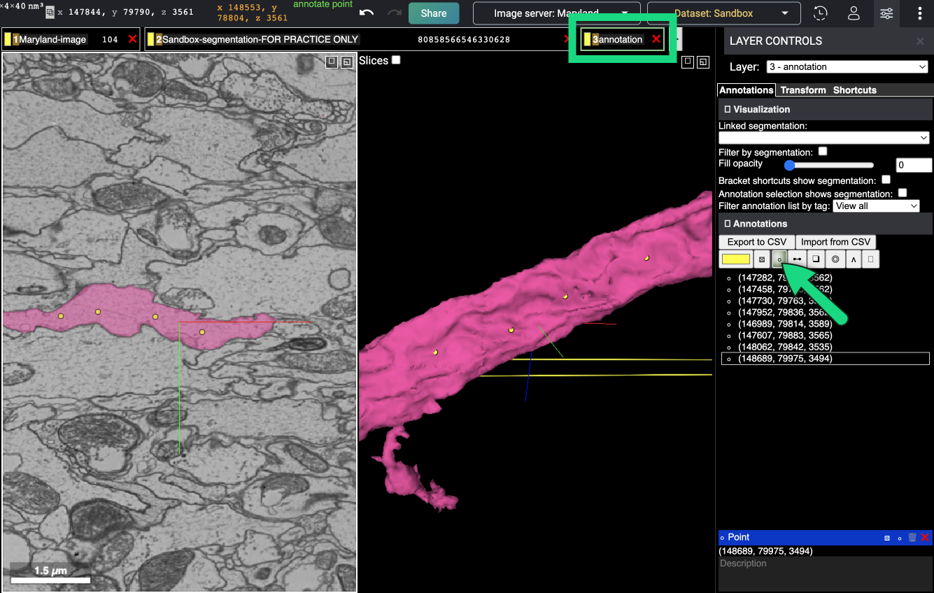
The annotation-interface image illustrates why coordinate provenance matters. A point can be meaningful only together with the imagery/segmentation context in which it was placed. In later lessons, you will use coordinates to resolve a location into a root ID at a specified materialization.

Create a single provenance object now. Store both the selected values and the complete materialization table that informed the choice.

COORDINATE_SYSTEM = {
    "axis_order": ["x", "y", "z"],
    "units": "nanometers",
    "native_voxel_resolution_nm": [4, 4, 40],
    "reference_volume": DATASTACK,
    "note": (
        "FlyWire API locations are recorded as physical x, y, z coordinates. "
        "Do not substitute voxel indices without an explicit conversion."
    ),
}

provenance = {
    "queried_utc": datetime.now(timezone.utc).isoformat(),
    "flywire_dataset_release": DATASET,
    "datastack": DATASTACK,
    "materialization_version": MATERIALIZATION_VERSION,
    "coordinate_system": COORDINATE_SYSTEM,
    "package_versions": {
        "caveclient": version("caveclient"),
        "fafbseg": version("fafbseg"),
        "pandas": version("pandas"),
    },
    "available_materializations_at_query_time": materializations.to_dict(
        orient="records"
    ),
    "datastack_info": datastack_info,
}

provenance

Finally, write it next to the notebook as JSON:

import json
from pathlib import Path

output_path = Path("flywire_provenance.json")

with output_path.open("w", encoding="utf-8") as f:
    json.dump(provenance, f, indent=2, default=str)

print(f"Wrote provenance to: {output_path.resolve()}")

The default=str option is deliberate: service metadata can contain timestamps or other Python objects that standard JSON cannot serialize directly.

---

A compact working pattern for future notebooks

At the beginning of each later notebook, either import the saved provenance or repeat the setup cell and create a new provenance file. For this course, prefer the second approach when starting a distinct project, because it reveals changes in package versions or available materializations.

Use this checklist before any neuron, annotation, or synapse query:

• The token is loaded from the environment, never notebook source.
• DATASET is explicit, normally "public" for this course.
• DATASTACK is recorded.
• One MATERIALIZATION_VERSION is selected from the live availability table.
• Every location is labeled as [x, y, z] in nanometers.
• flywire_provenance.json is saved with the notebook output.

Two common failures are worth recognizing:

Symptom	Likely cause	First response
Authentication or permission error	Missing, expired, or inaccessible token	Restart Jupyter from a shell with CAVE_TOKEN set; verify account access.
A later root-ID or synapse query cannot resolve	The root did not exist at the selected materialization, or dataset/materialization were mixed	Check the dataset and materialization first; do not switch to "auto" merely to suppress the error.
A location returns an implausible object	Coordinates were copied in a different unit or axis convention	Confirm x, y, z order and nanometer units before investigating biology.

At this stage, the notebook should be able to retrieve datastack metadata and list materializations, while producing a saved provenance record. That is sufficient. Resist the temptation to begin querying arbitrary root IDs before pinning a version.

---

You now have an authenticated, version-aware starting point for FlyWire analysis. The important distinction is that Public/Production/Sandbox selects a dataset context, while a materialization selects a reproducible snapshot of its annotation-related tables. Locations remain meaningful only when their coordinate order and units are recorded alongside that context.

Next, you will resolve a neuron identifier against the materialization you selected, so that later annotation and connectivity queries refer to a well-defined reconstructed object.