Autoregressive vs. Discrete Diffusion: Sequential and Parallel Token Generation

Hello. This first module establishes the conceptual shift underlying discrete diffusion language models: generation need not mean committing to tokens left-to-right. Instead, it can mean traversing a sequence-level probability path from simple noise to text.

In this lesson, you will contrast the two factorizations that create those very different decoding behaviors, identify exactly why ancestral autoregressive sampling is serial, and see why a discrete diffusion denoiser can update a whole token canvas in parallel. This is the foundation for the categorical Markov-chain mathematics and PyTorch corruption code in the next module.

A useful outcome for this session: you should be able to look at a decoding procedure and say whether its dependencies require token-by-token sampling, permit parallel token updates, or combine both.

---

1. Autoregressive generation: a dependency chain over positions

Let $c$ be a prompt and let $\mathbf{y}=(y_1,\dots ,y_L)$ denote the response tokens, including an end-of-sequence token that determines its length. A standard autoregressive language model defines

$$p_{\theta }(\mathbf{y}\mid c)=\prod _{i=1}^L{p}_{\theta }(y_i\mid y_{<i},c).$$

This is not merely a modeling convention: it dictates the exact ancestral sampling algorithm.

To sample $y_i$, we need a concrete sampled prefix $y_{<i}$. But to have that prefix, we must already have sampled every preceding token. Thus, for one generated sequence, the sampling dependency is inherently serial.

For example, suppose a response begins:

“The capital of France is …”

The model first samples “The,” then conditions on it to sample “capital,” then conditions on “The capital” to sample “of,” and so on. The next-token distribution is recalculated after each extension of the prefix.

A causal Transformer encodes this rule architecturally. At output position $i$, its attention mask permits attention to:

• the prompt tokens;
• response positions strictly to the left of $i$;
• not the yet-unsampled response positions to the right.

The model may compute training logits for all positions in parallel under teacher forcing, because the complete target sequence is already available. But that is not parallel generation. At inference time, those target tokens are unknown, and the sampled output at position $i$ becomes required input to position $i+1$.

The cost of serial dependence is not that autoregressive models are incapable of GPU parallelism. Within one forward pass, attention and matrix operations are highly parallel; batching also permits many different sequences to decode concurrently. The limitation is the number of dependent model evaluations for one sequence: a conventional sampler needs approximately one forward pass per generated token.

The benefit is equally important: the model’s distribution for each new token is directly conditioned on the exact, already committed prefix. That makes local continuation natural, but an early mistake is fed into all later steps. More fundamentally, the factorization gives no later position the ability to revise an earlier sampled token.

---

2. A discrete diffusion model defines a path through noisy sequences

Discrete diffusion starts from a different question. Rather than modeling “what is the next token?”, it defines a tractable way to gradually corrupt an entire clean sequence.

Let ${\mathbf{x}}_0$ be a clean token sequence. Introduce noisy versions

$${\mathbf{x}}_1,{\mathbf{x}}_2,\dots ,{\mathbf{x}}_T,$$

where the noise level increases with $t$. The forward process is a chosen Markov chain:

$$q({\mathbf{x}}_{1:T}\mid {\mathbf{x}}_0)=\prod _{t=1}^{T}q({\mathbf{x}}_t\mid {\mathbf{x}}_{t-1}).$$

This is the probability path. It is not an attempt to model plausible language while moving forward. It is deliberately designed to destroy linguistic information in a way whose probabilities we can calculate.

For categorical tokens, a usual design assigns a row-stochastic transition matrix $Q_t$ at each noise time. For one token position $j$, represented by a one-hot row vector,

$$q(x_t^{(j)}\mid x_{t-1}^{(j)})=\mathrm{Cat}\left(x_t^{(j)};x_{t-1}^{(j)}{Q}_t\right).$$

A simple masking process makes the intuition immediate:

• at $t=0$, the sequence is clean;
• at each forward step, an unmasked token can become $\text{[MASK]}$;
• after sufficient corruption, nearly every position is $\text{[MASK]}$.

The mask is an absorbing state in this particular forward process: once it is reached, further forward transitions leave it masked. Other discrete diffusion processes replace tokens with uniformly random vocabulary tokens instead; the next module will formalize that alternative.

For now, focus on what the path accomplishes. Instead of learning to generate from nothing in one step, the model learns to infer a clean sequence from partially damaged versions of it.

The cumulative effect of the forward matrices is

$${\overline{Q}}_t=Q_1{Q}_2\cdots Q_t.$$

Therefore the marginal corruption distribution at time $t$ can be sampled directly:

$$q(x_t^{(j)}\mid x_0^{(j)})=\mathrm{Cat}\left(x_t^{(j)};x_0^{(j)}{\overline{Q}}_t\right).$$

This is already a major engineering advantage. We can take a clean training sentence, select a noise level $t$, and corrupt it to that level directly. We do not need to simulate all preceding forward steps.

---

3. Reverse denoising: dependencies are over noise levels, not token positions

Generation reverses the corruption path. The learned model is written as

$$p_{\theta }({\mathbf{x}}_{0:T}\mid c)=p({\mathbf{x}}_T)\prod _{t=1}^T{p}_{\theta }({\mathbf{x}}_{t-1}\mid {\mathbf{x}}_t,c).$$

Here, $p({\mathbf{x}}_T)$ is a simple terminal distribution, such as all masks or a uniform categorical distribution. Generation begins there and visits progressively less noisy states until it obtains ${\mathbf{x}}_0$.

The key difference from autoregression is where the conditioning sits:

Model family	Conditional distribution at one generation step	Required sequence of decisions
Autoregressive	$p_{\theta }(y_i\mid y_{<i},c)$	Positions $1,2,\dots ,L$
Discrete diffusion	$p_{\theta }({\mathbf{x}}_{t-1}\mid {\mathbf{x}}_t,c)$	Noise levels $T,T-1,\dots ,0$

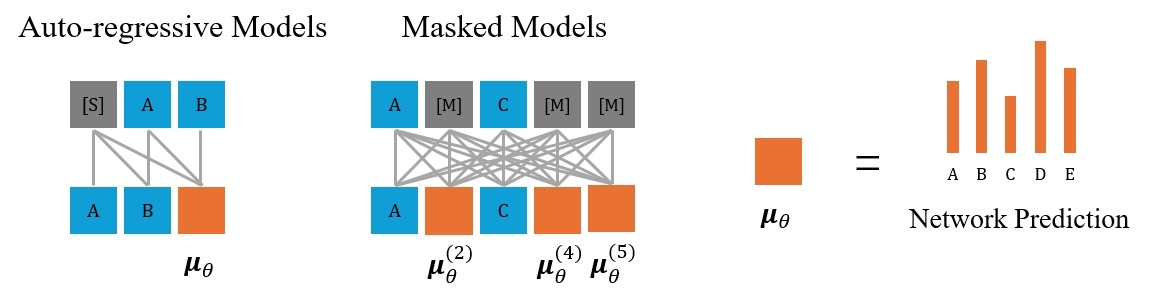
An autoregressive step creates one new position, conditioned on a sampled prefix. A diffusion step receives a whole current canvas ${\mathbf{x}}_t$, perhaps containing masks or corrupted tokens, and predicts a less-noisy whole canvas.

A practical denoiser typically produces vocabulary logits at every position simultaneously:

$${\tilde{p}}_{\theta }\left(x_0^{(j)}\mid {\mathbf{x}}_t,t,c\right)=\mathrm{Softmax}\left(f_{\theta }({\mathbf{x}}_t,t,c{)}_j\right).$$

The notation reveals two important facts.

First, every position $j$ receives a prediction in one Transformer evaluation. There is no requirement to sample position $j-1$ before calculating the distribution at $j$.

Second, this does not mean the model regards positions as unrelated. With bidirectional attention over the denoising canvas, the representation used for one position can depend on the current noisy tokens at all the other positions. A partially recovered phrase on the right can influence an uncertain token on the left, while the prompt constrains the entire canvas.

This is the central dependency contrast:

• AR dependency: token $y_i$ depends on realized earlier output tokens, so an exact sampler must wait for those tokens.
• Diffusion dependency: the next canvas depends on the already available current canvas ${\mathbf{x}}_t$, so all positions can be updated during the same denoising evaluation.
• Remaining serial dependency in diffusion: denoising time steps still occur sequentially. Parallel token updates do not imply that the entire response emerges in one forward pass.

A useful mental model is that autoregression builds a sentence by extending one committed boundary, whereas diffusion maintains a mutable draft at a chosen set of positions and repeatedly improves that draft.

---

4. Why parallel updates are possible, and what they do not guarantee

Consider an initial diffusion canvas of five masks:

$${\mathbf{x}}_T=[\text{[MASK]},\text{[MASK]},\text{[MASK]},\text{[MASK]},\text{[MASK]}].$$

At a reverse step, the denoiser can produce five vocabulary distributions at once. For a prompt such as “Complete: Paris is the capital of …”, different positions might acquire high-confidence candidates such as “France” and an end token, while other positions remain uncertain.

Sampling or accepting several positions at that same reverse step is legal because none requires a newly sampled neighbor from that same step as input. Each uses the shared prior canvas ${\mathbf{x}}_t$.

This parallelism depends on three design choices:

1. A sequence-level state exists.
   The sampler maintains ${\mathbf{x}}_t$, not merely a generated prefix and an unknown suffix.

2. The denoiser has simultaneous access to that state.
   In a pure diffusion canvas, bidirectional attention can let a masked location attend to tokens on either side.

3. The reverse update is conditionally parallelizable.
   The implementation may sample coordinate-wise from predicted categorical distributions, or decide which locations to reveal together. The model has already computed all these distributions in one pass.

However, “parallel” must not be confused with “independent.”

At the beginning, when every location is masked, a model cannot rely on revealed neighboring text. It must use the prompt, position information, and its learned distribution over complete sequences. Early parallel proposals can conflict: independently proposed words may not agree on syntax, entity identity, or sentence length. Later reverse steps condition on the evolving shared canvas and can resolve some inconsistencies.

This is how diffusion can represent strongly correlated language despite parallel per-position predictions: dependencies are mediated through repeated, globally contextualized denoising steps. The exact reverse distribution over a whole sequence can be complex; practical models choose parameterizations that make each step tractable.

The distinction matters for performance claims, too. If a diffusion sampler requires $20$ denoising evaluations but resolves an average of $8$ useful tokens per evaluation, it may reduce latency relative to $160$ autoregressive token evaluations. But a naïve parallel update that needs many refinement steps, or produces weak drafts, may not win. The relevant unit is not “tokens predicted per pass,” but high-quality tokens finalized per pass. Later we will implement and measure this tradeoff.

The refinement shown in the figure highlights a practical nuance. In basic absorbing-mask diffusion, a reverse sampler often treats revealed tokens as committed: a token that has been unmasked is not remasked in later steps. That makes decoding simple but allows an early incorrect commitment to persist. More flexible samplers can re-noise low-confidence proposals, restoring the ability to revise a draft. The mechanics and tradeoffs of that choice belong to the sampler modules later in the course.

---

5. A compact comparison to retain

When deciding whether a generation scheme can update tokens in parallel, ask one question:

Does predicting a token require a newly sampled token from this same output sequence, or only the already available state from the previous iteration?

Property	Autoregressive LM	Discrete diffusion LM
Object modeled during generation	Growing prefix	Entire noisy sequence
Natural attention pattern over generated output	Causal	Bidirectional within denoising canvas
Serial dimension	Token position	Denoising time
Tokens proposed per network evaluation	Usually one per sequence	Potentially many
Can a later step revise an earlier token?	Not in ordinary ancestral sampling	Potentially yes, depending on the noise and sampling design
Simple terminal state	Empty prefix plus prompt	All masks or categorical noise
Major decoding challenge	Long sequential chain	Coherent, efficient iterative refinement

The forward diffusion process is intentionally simple and known. The reverse process is where language modeling happens. Training will teach a neural network to infer clean tokens from corrupted contexts; sampling will use that network repeatedly to traverse from noise back toward text.

---

Key takeaways

Autoregressive and diffusion language models define different probability factorizations:

$$p_{\theta }(\mathbf{y}\mid c)=\prod _i{p}_{\theta }(y_i\mid y_{<i},c)$$

forces serial token sampling because each new token requires a realized prefix.

$$p_{\theta }({\mathbf{x}}_{0:T}\mid c)=p({\mathbf{x}}_T)\prod _t{p}_{\theta }({\mathbf{x}}_{t-1}\mid {\mathbf{x}}_t,c)$$

moves serial dependence to denoising time. At each time, the model receives an entire existing noisy canvas, so it can calculate updates for many positions in parallel.

The price is iterative refinement: diffusion is not one-shot generation, and parallel proposals are not automatically coherent. The payoff is a different computational and modeling interface—one that can use bidirectional context and potentially revise uncertain parts of a developing answer.

Next, we will make the forward probability path concrete. You will derive the transition kernel for a uniform-replacement categorical continuous-time Markov chain, calculate its noisy token marginals, and implement vectorized token corruption in PyTorch.