
Hello! Welcome to your next lesson.
In our last session, you implemented a streaming inference loop, learning how to process audio incrementally with frame-synchronous CTC decoders. This gave you the "how" of building a real-time system. Today, we address the critical next question: "Why is it slow?"
This lesson focuses on a crucial skill for any systems-focused AI developer: performance analysis. Our learning outcome is to analyze the performance bottlenecks in a typical speech AI inference pipeline. We'll move beyond just the model to dissect the entire system—from data input to final output—to identify and understand what's limiting performance.
1. The Anatomy of a Speech AI Pipeline
Before we can find a bottleneck, we need a map of the system. A speech AI pipeline isn't a single monolithic block; it's a sequence of stages, and latency accumulates at each step.
A helpful way to visualize this is as a "latency funnel."
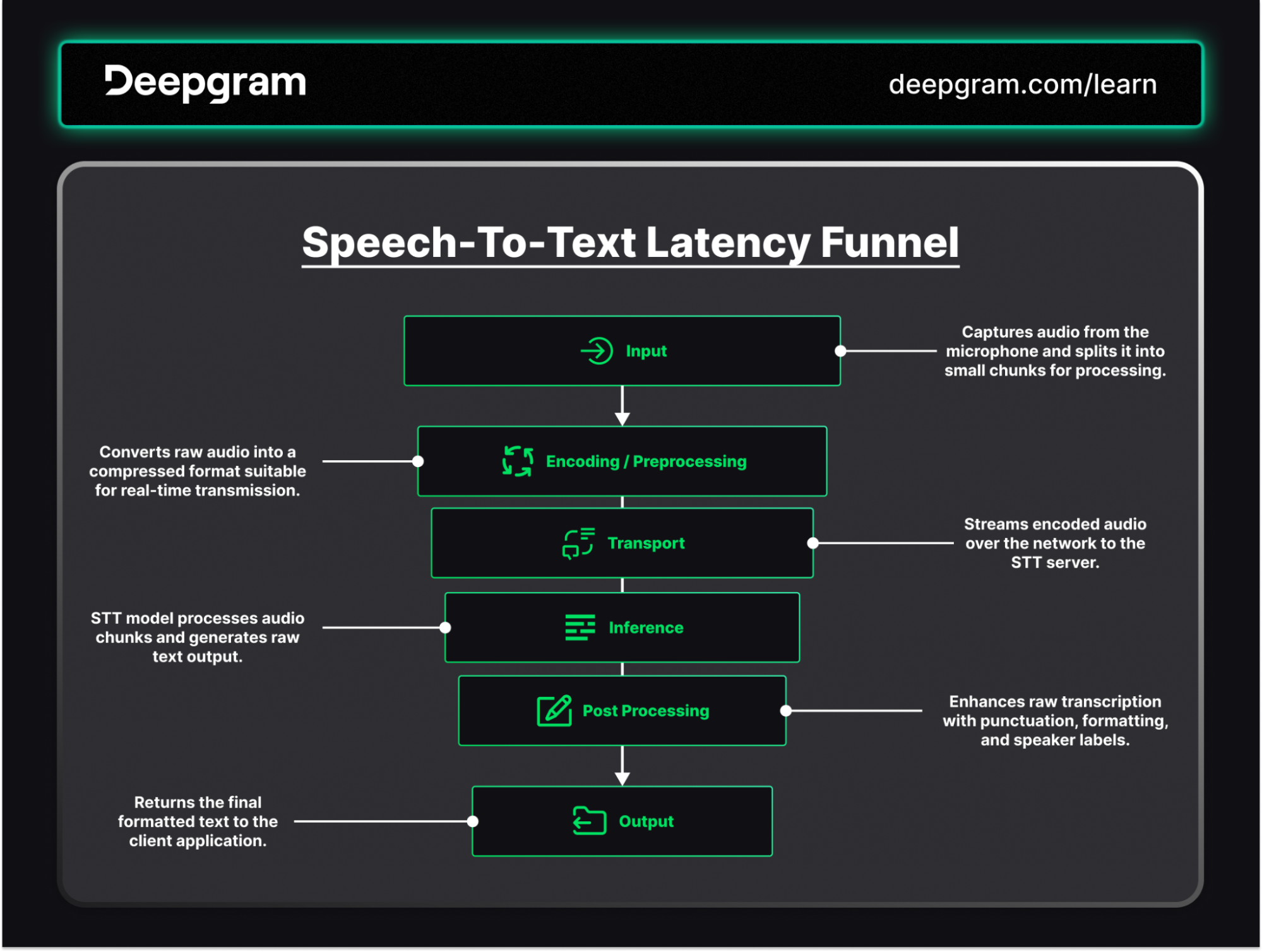
Understanding and Reducing Latency in Speech-to-Text APIs
To understand these stages in more detail, let's read an article from Deepgram that breaks down the sources of latency.
Read the sections 'What are the sources of latency in STT APIs?' and 'Latency Funnel Breakdown: Where Do The Milliseconds Hide?'. As you read, map these stages to your own experience with ASR systems. Note how many potential failure points exist outside of the core model inference.
As the article highlights, the total latency is a chain, and it's only as strong as its weakest link. A lightning-fast model is useless if it's starved for data or if network transport is slow.
2. Conceptual Frameworks for Bottleneck Analysis
When analyzing a pipeline, we're often looking for specific anti-patterns. A real-world case study can provide a powerful mental model for identifying these issues.
Optimizing Latency in Real-Time Speech Translation Pipelines
This article from Webline Global details a real-world project where a speech translation pipeline failed due to high latency. Their analysis reveals several classic architectural bottlenecks.
Read the sections 'WHAT WENT WRONG' and 'HOW WE APPROACHED THE SOLUTION'. Pay close attention to the three primary bottlenecks they identified and the conceptual shift they adopted.
From this case study, we can extract three critical concepts for analyzing any real-time pipeline:
- The Waterfall Trap: This is the most common bottleneck. The system is designed as a strict sequence (e.g., ASR → MT → TTS), and the total latency is the sum of each component's processing time. Each stage must wait for the previous one to fully complete.
- Blocking Dependencies: A specific form of the waterfall trap where one stage actively blocks another. The article's example of the ASR model waiting for the Language ID (LID) model to finish is a perfect illustration.
- Store-and-Process vs. Stream-and-Compute: This is the fundamental mindset shift required for low-latency systems.
- Store-and-Process: Wait for a complete unit of work (e.g., a full sentence), then process it. This maximizes accuracy but also latency.
- Stream-and-Compute: Process data as it arrives, passing partial results downstream immediately. This is the "bucket brigade" analogy from the article and is the essence of the streaming loops we built in the last lesson.
Your goal as a systems analyst is to identify where your pipeline falls into the "waterfall" or "store-and-process" traps and re-architect it towards a "stream-and-compute" model.
3. The Tool for the Job: PyTorch Profiler
To move from concepts to code, we need a tool to measure what's happening. For PyTorch models, the built-in profiler (torch.profiler) is indispensable. Given your extensive PyTorch experience, this tool will feel like a natural extension of your workflow.
Debugging and Optimization of PyTorch Models
This comprehensive tutorial from Sharcnet HPC provides a masterclass in using the PyTorch Profiler. We'll use it to understand how to pinpoint CPU, GPU, and memory bottlenecks.
Please watch the following segments: Why Profile? (01:29 - 02:53): Understand the motivation behind profiling. When to Profile (02:53 - 05:09): Learn the strategic points in development to use the profiler. Basic Usage (05:09 - 08:38): See how to wrap your code with the profiler context manager and generate basic summary tables. Case Study: GPU Idle Time (08:38 - 19:26): This is the most critical section. It demonstrates how to export a trace, view it in Chrome, and identify a classic data-loading bottleneck where the GPU is idle, waiting for the CPU. Pay close attention to how increasing num_workers in the DataLoader helps resolve this.
Key Profiling Insights for Speech Pipelines
The video gives us a powerful methodology. Let's apply it to our domain.
Bottleneck #1: CPU-Bound Data Pipeline (GPU Starvation)
As the case study in the video demonstrated, one of the most common bottlenecks is the GPU waiting for the CPU. In a speech pipeline, this can manifest in several ways:
- During Training/Batch Inference: The
DataLoaderis too slow. This could be due to complex on-the-fly augmentations, slow disk I/O, ornum_workers=0. The PyTorch profiler's trace view will show large gaps in the "GPU Util" track, corresponding to CPU activity in thedataloadertrack. - During Real-time Inference: The CPU is responsible for audio I/O, resampling, and feature extraction (like STFT or Mel-spectrograms) before the data even reaches the GPU. If these steps, running on the CPU, take longer than the model inference on the GPU, the GPU will be starved.

Bottleneck #2: Memory Issues
The profiler can also track memory usage, which is crucial for identifying two types of problems:
- Out-of-Memory (OOM) Errors: The most obvious issue. Profiling can show you exactly which operation allocates the tensor that pushes you over the memory limit.
- Memory Leaks: A more insidious problem where memory usage grows over time, eventually leading to a crash.
Debugging and Optimization of PyTorch Models
Let's continue with the 'Debugging and Optimization of PyTorch Models' video to see how to diagnose memory issues.
Watch the section on memory profiling (23:13 - 27:17). The example shows a memory leak caused by not clearing gradients in a training loop. This same principle applies to inference: if you unintentionally hold onto tensors from previous requests, memory will grow indefinitely.
4. Analyzing Streaming-Specific Bottlenecks
While the PyTorch profiler is a general tool, streaming systems have unique characteristics. A non-streaming batch ASR job might be bottlenecked by data loading, but a live streaming server faces different challenges.
Inference Characteristics of Streaming Speech Recognition
This video, 'Inference Characteristics of Streaming Speech Recognition', analyzes the performance of a real-world open-source streaming ASR server. It highlights bottlenecks unique to this setting.
Watch these key sections: Memory Behavior (05:17 - 06:11): Notice how GPU memory is stable, but CPU memory grows with the number of concurrent connections. KV Cache Eviction (06:11 - 08:18): This is a critical concept. To prevent memory from growing forever in a long-running stream, the model's KV cache (its state) must be intelligently pruned. A failure to do this is a memory bottleneck. Faster-than-Real-Time Input (08:18 - 08:58): See what happens when the client sends audio faster than the server can process it. The input buffer on the CPU grows without bound, leading to a crash. This is a classic producer-consumer problem. Comparison to LLMs (10:09 - 11:40): This summary contrasts the challenges of streaming ASR (stateful, long connections) with LLM inference, reinforcing the unique bottlenecks we face.
This video introduces us to the Real-Time Factor (RTF), an implicit but vital metric. It's the ratio of the time it takes to process an audio segment to the duration of the audio segment itself.
For a system to be "real-time," the RTF must be less than 1. The processing time includes all stages: CPU pre-processing, GPU inference, and CPU post-processing. The profiler is your tool to measure the total processing time and break it down to see which component is contributing most to an RTF > 1.
5. A Checklist for Performance Analysis
When faced with a slow speech pipeline, here is a systematic approach to finding the bottleneck:
- Establish a Baseline: Measure your end-to-end latency and calculate your RTF.
- Profile the Pipeline: Use
torch.profilerto generate a trace. - Analyze GPU Utilization:
- Is the GPU idle for long periods? If yes, you are CPU-bound or I/O-bound.
- Look at the CPU-side operations in the trace: data loading, pre-processing (feature extraction), post-processing (decoding, formatting).
- If training, increase
DataLoadernum_workers. - If doing real-time inference, check network I/O and CPU-based feature extraction.
- Is the GPU idle for long periods? If yes, you are CPU-bound or I/O-bound.
- Analyze GPU Active Time:
- Is the GPU fully utilized but the RTF is still > 1? If yes, you are GPU-bound (compute-bound).
- The model itself is the bottleneck. The operations within the forward pass are too slow.
- This is the signal to begin model optimization techniques like quantization, knowledge distillation, or using
torch.compile(), which we will cover in the next module.
- Is the GPU fully utilized but the RTF is still > 1? If yes, you are GPU-bound (compute-bound).
- Analyze Memory Usage:
- Does memory usage grow over time? If yes, you have a memory leak.
- In streaming models, check your KV cache management. Is old state being evicted correctly?
- In any pipeline, ensure you are not holding onto tensors from previous requests or batches (e.g., in a global list).
- Does the application crash with an OOM error? Use the memory profiler to pinpoint the exact operation that allocates the large tensor. The solution might be to reduce batch size or use a smaller model.
- Does memory usage grow over time? If yes, you have a memory leak.
Conclusion
In this lesson, you've learned to think like a systems engineer, dissecting a speech AI pipeline to find its weakest links. You now have both a conceptual framework and a practical toolkit for performance analysis.
Key Takeaways:
- Speech AI pipelines are multi-stage systems, and latency is cumulative. Common bottlenecks include data I/O, CPU pre-processing, model compute, and architectural design.
- The "Waterfall Trap"—where processing is strictly sequential—is a major anti-pattern. The goal is to move towards a "Stream-and-Compute" model.
torch.profileris the essential tool for identifying bottlenecks. By visualizing CPU/GPU activity in a trace, you can diagnose whether your system is CPU-bound, I/O-bound, or compute-bound.- Streaming systems have unique challenges, such as managing the stateful KV cache to prevent memory growth and handling producer-consumer imbalances between the client and server.
- Performance analysis is a systematic process: measure, profile, identify the limiting factor (CPU, GPU, memory, I/O), and then apply a targeted solution.
Preview of the Next Lesson:
You've now learned how to identify a compute-bound bottleneck, where the model itself is simply too slow. What do you do next? The next module, Model Optimization for Deployment, provides the answers. In our first lesson, we will explore knowledge distillation, a powerful technique to compress a large, slow model into a smaller, faster "student" model without a significant loss in accuracy.