Backpropagation from Scratch

Hello! Let's dive into the second lesson of our "Deep Neural Network Fundamentals" module.

Introduction

In our previous lesson, we successfully built a multi-layer perceptron (MLP) and implemented forward propagation. This gave our network the ability to take an input, like a handwritten digit, and produce a prediction. However, since we initialized the network's weights and biases randomly, these predictions are, for now, completely meaningless.

Today, we will answer the crucial question: How does a neural network learn from its mistakes?

The answer lies in the celebrated backpropagation algorithm. This lesson is dedicated to understanding, deriving, and implementing backpropagation from scratch. It is arguably the most important algorithm in deep learning, as it enables our networks to learn complex patterns from data. Backpropagation is essentially a highly efficient method for applying the chain rule from calculus to compute the gradient of the loss function with respect to every single weight and bias in the network. Once we have these gradients, we can use them to "nudge" our parameters in the right direction to improve the network's performance.

By the end of this lesson, you will be able to derive the backpropagation algorithm from first principles and implement it in Python to train your first neural network.

1. The Core Idea: Gradient Descent and the Chain Rule

Before diving into the math, let's establish the high-level goal. We have:

1. A network that makes a prediction $\hat{y}$ from an input $\mathbf{x}$.
2. A loss function $L(\hat{y},y)$ that measures how far our prediction is from the true label $y$.

Our goal is to adjust the network's parameters (weights $\mathbf{W}$ and biases $\mathbf{b}$) to minimize this loss. The most common way to do this is with gradient descent. We calculate the gradient of the loss with respect to each parameter—a vector that points in the direction of the steepest ascent of the loss—and take a small step in the opposite direction.

$$\text{parameter}\leftarrow \text{parameter}-\alpha \cdot \frac{\partial L}{\partial \text{parameter}}$$

Here, $\alpha$ is the learning rate. The challenge is calculating the partial derivatives (e.g., $\frac{\partial L}{\partial w_{ij}^{[l]}}$) for potentially millions of parameters in a deep network. This is where backpropagation comes in. It's an algorithm that computes these gradients efficiently by propagating the error signal backward through the network, from the output layer to the input layer.

2. Intuition and Calculus of Backpropagation

At its heart, backpropagation is a clever application of the chain rule. To build a strong intuition for this, there's no better resource than the one from 3Blue1Brown.

A More Formal Derivation

Now, let's formalize the concepts from the video using the notation from our previous lesson. The core of backpropagation is computing the gradient of the loss $L$ with respect to the parameters of each layer $l$. This boils down to finding $\frac{\partial L}{\partial W^{[l]}}$ and $\frac{\partial L}{\partial b^{[l]}}$.

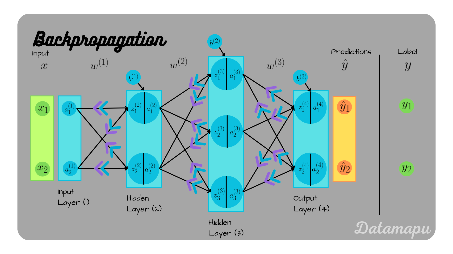
The chain rule tells us that to find the gradient with respect to a weight $W^{[l]}$, we can write:

$$\frac{\partial L}{\partial W^{[l]}}=\frac{\partial L}{\partial Z^{[l]}}\frac{\partial Z^{[l]}}{\partial W^{[l]}}$$

Let's break this down:

1. $\frac{\partial Z^{[l]}}{\partial W^{[l]}}$: Since $Z^{[l]}=W^{[l]}{A}^{[l-1]}+b^{[l]}$, the derivative of $Z^{[l]}$ with respect to $W^{[l]}$ is simply $A^{[l-1]}$.
2. $\frac{\partial L}{\partial Z^{[l]}}$: This term is the error signal for layer $l$, often denoted as ${\delta }^{[l]}$. It tells us how the final loss is affected by the pre-activation values in layer $l$.

The brilliance of backpropagation is how it computes ${\delta }^{[l]}$ for every layer recursively, starting from the last layer, $L$.

• For the Output Layer ($l=L$):
  ${\delta }^{[L]}=\frac{\partial L}{\partial Z^{[L]}}=\frac{\partial L}{\partial A^{[L]}}\odot g^{\prime [L]}(Z^{[L]})$
  where $\odot$ is element-wise multiplication and $g^{\prime [L]}$ is the derivative of the activation function of the output layer.

• For any Hidden Layer ($l<L$):
  The error at layer $l$ depends on the error from layer $l+1$.
  ${\delta }^{[l]}=\frac{\partial L}{\partial Z^{[l]}}=\left((W^{[l+1]}{)}^T{\delta }^{[l+1]}\right)\odot g^{\prime [l]}(Z^{[l]})$
  This is the "propagation" rule: the error from the next layer (${\delta }^{[l+1]}$) is multiplied by the weights connecting the layers ($(W^{[l+1]}{)}^T$) and then by the local gradient of the activation function.

Once we have ${\delta }^{[l]}$ for a given layer, the gradients for the parameters of that layer are straightforward:

$$\frac{\partial L}{\partial W^{[l]}}={\delta }^{[l]}(A^{[l-1]}{)}^T$$ $$\frac{\partial L}{\partial b^{[l]}}=\text{np.sum}({\delta }^{[l]},\text{axis=1, keepdims=True})$$

(We sum the errors across all examples in the batch for the bias gradient).

For a detailed, step-by-step mathematical derivation, the following article is an excellent resource.

3. Implementing Backpropagation with NumPy

Now we'll translate this theory into code, continuing with the MLP we started in the last lesson. We'll follow the structure of the Samson Zhang video, which we also used for forward propagation.

Step 3.1: The back_prop Function

The back_prop function will take the activations and parameters from the forward pass, along with the true labels, and compute the gradients for all weights and biases.

A crucial simplification occurs when using Softmax activation with Cross-Entropy Loss (which is standard for multi-class classification). The derivative of the loss with respect to the final pre-activation, $\frac{\partial L}{\partial Z^{[L]}}$, simplifies beautifully to:

$${\delta }^{[L]}=A^{[L]}-Y$$

where $A^{[L]}$ is the matrix of predicted probabilities and $Y$ is the one-hot encoded matrix of true labels. This avoids calculating the complex derivatives of Softmax and the loss function separately.

We also need the derivative of our hidden layer activation, ReLU:

$${\text{ReLU}}^{\prime }(z)=\{\begin{array}{ll}1& \text{if }z>0\\ 0& \text{if }z\le 0\end{array}$$

Now, we can write our back_prop function.

# Based on the video's implementation

def one_hot(Y):
    # Creates a one-hot encoded matrix of the labels
    one_hot_Y = np.zeros((Y.size, Y.max() + 1))
    one_hot_Y[np.arange(Y.size), Y] = 1
    one_hot_Y = one_hot_Y.T
    return one_hot_Y

def deriv_ReLU(Z):
    # Returns 1 for Z > 0, 0 otherwise
    return Z > 0

def back_prop(Z1, A1, Z2, A2, W2, X, Y):
    m = Y.size # Number of training examples
    one_hot_Y = one_hot(Y)
    
    # Layer 2 gradients
    dZ2 = A2 - one_hot_Y
    dW2 = 1 / m * dZ2.dot(A1.T)
    db2 = 1 / m * np.sum(dZ2, axis=1, keepdims=True)
    
    # Layer 1 gradients
    dZ1 = W2.T.dot(dZ2) * deriv_ReLU(Z1)
    dW1 = 1 / m * dZ1.dot(X.T)
    db1 = 1 / m * np.sum(dZ1, axis=1, keepdims=True)
    
    return dW1, db1, dW2, db2

The back_prop function implements the equations we derived. It starts from the output layer (dZ2) and works backward to compute all gradients.

Step 3.2: The update_params Function

This function is simple: it takes the current parameters and the computed gradients and performs the gradient descent step.

def update_params(W1, b1, W2, b2, dW1, db1, dW2, db2, alpha):
    W1 = W1 - alpha * dW1
    b1 = b1 - alpha * db1
    W2 = W2 - alpha * dW2
    b2 = b2 - alpha * db2
    return W1, b1, W2, b2

This function applies the gradient descent update rule to each parameter.

You can follow along with the video's implementation of these functions.

Test your understanding!

In our back_prop function, we calculate dZ1 = W2.T.dot(dZ2) * deriv_ReLU(Z1).
In terms of our formal derivation, which part of the equation ${\delta }^{[l]}=\left((W^{[l+1]}{)}^T{\delta }^{[l+1]}\right)\odot g^{\prime [l]}(Z^{[l]})$ does each part of the code correspond to?
(Here, $l=1$).

Show answer

• W2.T: This corresponds to $(W^{[2]}{)}^T$.
• dZ2: This is the error signal from the next layer, ${\delta }^{[2]}$.
• W2.T.dot(dZ2): This corresponds to the term $(W^{[2]}{)}^T{\delta }^{[2]}$.
• *: This is the element-wise multiplication, $\odot$.
• deriv_ReLU(Z1): This is the derivative of the activation function for layer 1, $g^{\prime [1]}(Z^{[1]})$.

The code is a direct implementation of the backpropagation rule for a hidden layer.

A Deeper Look: The Computational Graph

Your computer science background gives you a unique advantage in understanding a deeper, more fundamental view of backpropagation. Modern frameworks like PyTorch and TensorFlow don't just see a "network"; they see a computational graph. Every operation (addition, multiplication, tanh, etc.) is a node in this graph.

Forward propagation is the process of evaluating this graph. Backpropagation is simply applying the chain rule recursively over this graph, starting from the final output node.

The article below implements a Value object that mimics this behavior. It's a fantastic way to truly grasp how automatic differentiation (autograd) engines work from the ground up.

This perspective connects the high-level math of backpropagation directly to the low-level implementation details found in professional deep learning frameworks.

Conclusion

Fantastic work! Today, you've conquered one of the most fundamental and powerful concepts in deep learning. By deriving and implementing backpropagation, you've built a neural network that can actually learn from data.

Key Takeaways:

• Backpropagation is an efficient algorithm for computing the gradient of the loss function with respect to all network parameters.
• It works by applying the chain rule recursively, starting from the output layer and moving backward.
• The algorithm consists of a forward pass (to compute activations and loss) and a backward pass (to compute gradients).
• The core of the backward pass is the recursive calculation of the error signals (${\delta }^{[l]}$) for each layer.
• Once gradients are computed, we use an optimization algorithm like gradient descent to update the network's weights and biases, moving the network toward a state of lower loss.

Preview of the next lesson:
Now that we have a working training pipeline, we can start refining our network. In the next lesson, we will take a closer look at the tools in our toolbox: the activation functions. We'll compare the properties and use cases of common functions like Sigmoid, Tanh, ReLU, and Leaky ReLU, and understand why the choice of activation function is so important for training deep networks.