Frequency Response and Decibel Analysis of First-Order RC Circuits

Good to see you again. In the previous lesson, you analyzed RC circuits in the time domain: capacitor voltage changed exponentially, and the time constant was $\tau =RC$ or, more generally, $R_{\mathrm{Th}}C$. The same $RC$ product now controls a different question: how does the circuit respond after a sinusoid has been applied long enough for transients to disappear?

This lesson develops the sinusoidal steady-state response of first-order RC low-pass and high-pass circuits. You will use complex impedance and voltage division to obtain a transfer function, calculate output magnitude and phase at any frequency, identify the cutoff frequency, and express voltage or power ratios in decibels. These are the exact tools later used to estimate amplifier bandwidth and interpret AC simulations.

---

From a sinusoid to a frequency response

Consider a sinusoidal input

$$v_{\mathrm{in}}(t)=V_m\cos (\omega t+{\varphi }_{\mathrm{in}})$$

where $\omega$ is angular frequency in radians per second:

$$\omega =2\pi f$$

and $f$ is frequency in hertz.

For a linear circuit containing resistors and capacitors, once initial transient behavior has died out, the output is also sinusoidal at the same frequency. Its amplitude and phase can differ:

$$v_{\mathrm{out}}(t)=|H(j\omega )|V_m\cos \left(\omega t+{\varphi }_{\mathrm{in}}+\angle H(j\omega )\right)$$

The complex quantity

$$H(j\omega )=\frac{{\tilde{V}}_{\mathrm{out}}}{{\tilde{V}}_{\mathrm{in}}}$$

is the transfer function evaluated at sinusoidal frequency $\omega$. It contains two pieces of information:

• $|H(j\omega )|$: output amplitude divided by input amplitude.
• $\angle H(j\omega )$: output phase relative to input phase.

A transfer function is not merely a single gain value. It is a function of frequency.

The key transition from the previous lesson is this:

• In DC steady state, a capacitor behaves as an open circuit.
• In sinusoidal steady state, a capacitor is represented by a frequency-dependent complex impedance.

$$Z_R=R$$ $$Z_C=\frac{1}{j\omega C}=-\frac{j}{\omega C}$$

The magnitude of capacitive impedance is

$$|Z_C|=\frac{1}{\omega C}$$

Thus, as frequency increases, a capacitor’s impedance magnitude falls. This one fact explains the behavior of both RC low-pass and high-pass filters.

---

RC low-pass filter: output taken across the capacitor

In the standard RC low-pass circuit, a resistor is in series with the source and a capacitor connects from the output node to the reference node. The output voltage is the capacitor voltage.

Because $R$ and $Z_C$ are in series, use the impedance form of the voltage-divider rule:

$$H_{\mathrm{LP}}(j\omega )=\frac{{\tilde{V}}_{\mathrm{out}}}{{\tilde{V}}_{\mathrm{in}}}=\frac{Z_C}{R+Z_C}$$

Substitute the capacitor impedance:

$$H_{\mathrm{LP}}(j\omega )=\frac{\frac{1}{j\omega C}}{R+\frac{1}{j\omega C}}$$

Multiply the numerator and denominator by $j\omega C$:

$$H_{\mathrm{LP}}(j\omega )=\frac{1}{1+j\omega RC}$$

This compact equation is worth recognizing immediately. It has one pole and therefore describes a first-order low-pass response.

Magnitude

For a complex number $a+jb$,

$$|a+jb|=\sqrt{a^2+b^2}$$

Therefore,

$$\left|1+j\omega RC\right|=\sqrt{1+(\omega RC{)}^2}$$

The magnitude response is

$$\boxed{\left|H_{\mathrm{LP}}(j\omega )\right|=\frac{1}{\sqrt{1+(\omega RC{)}^2}}}$$

Phase

The numerator of $H_{\mathrm{LP}}$ has phase $0^{\circ }$. The denominator has phase

$${\tan }^{-1}(\omega RC)$$

Since phase in a denominator is subtracted,

$$\boxed{\angle H_{\mathrm{LP}}(j\omega )=-{\tan }^{-1}(\omega RC)}$$

The negative phase means the output voltage lags the input voltage.

Physical checks

Always check a transfer function at extreme frequencies.

At low frequency,

$$\omega \to 0$$ $$Z_C\to \infty$$

The capacitor is nearly open, so there is almost no current through $R$, almost no drop across $R$, and the output follows the input:

$$|H_{\mathrm{LP}}|\to 1$$ $$\angle H_{\mathrm{LP}}\to 0^{\circ }$$

At very high frequency,

$$\omega \to \infty$$ $$Z_C\to 0$$

The capacitor increasingly pulls the output node toward the reference node:

$$|H_{\mathrm{LP}}|\to 0$$ $$\angle H_{\mathrm{LP}}\to -90^{\circ }$$

So low-frequency signals pass with little attenuation, whereas high-frequency signals are attenuated. Hence the name low-pass filter.

---

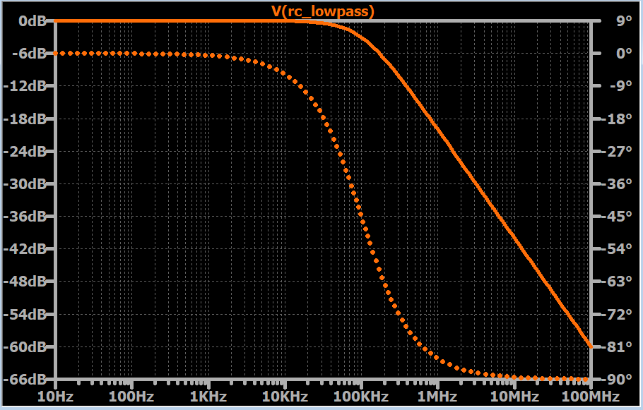
Cutoff frequency and its link to the time constant

The corner, break, or cutoff angular frequency of a simple RC filter is

$$\boxed{{\omega }_c=\frac{1}{RC}}$$

Since $\tau =RC$,

$${\omega }_c=\frac{1}{\tau }$$

Converting to hertz gives

$$\boxed{f_c=\frac{1}{2\pi RC}}$$

At cutoff,

$$\omega ={\omega }_c$$

so

$$\omega RC=1$$

The low-pass magnitude becomes

$$|H_{\mathrm{LP}}(j{\omega }_c)|=\frac{1}{\sqrt{2}}\approx 0.707$$

and the phase is

$$\angle H_{\mathrm{LP}}(j{\omega }_c)=-{\tan }^{-1}(1)=-45^{\circ }$$

At this frequency,

$$|Z_C|=R$$

The resistor and capacitor have equal impedance magnitudes, which is a useful quick check.

The amplitude is not “cut off” abruptly at $f_c$. It has fallen to $70.7\%$ of its low-frequency value. The word cutoff is conventional; the response continues smoothly beyond this frequency.

---

Decibels: voltage ratios versus power ratios

Frequency responses often span ratios ranging from nearly one down to tiny values. Decibels make such changes easier to calculate and plot.

For a voltage or current ratio, use

$$\boxed{G_{\mathrm{dB}}=20{\log }_{10}\left|\frac{V_{\mathrm{out}}}{V_{\mathrm{in}}}\right|}$$

For a power ratio, use

$$\boxed{G_{P,\mathrm{dB}}=10{\log }_{10}\left(\frac{P_{\mathrm{out}}}{P_{\mathrm{in}}}\right)}$$

The different factors, $20$ and $10$, matter. Power is proportional to the square of voltage only when the relevant resistances are equal:

$$P=\frac{V_{\mathrm{rms}}^2}{R}$$

Thus, when input and output are measured across equal resistances,

$$\frac{P_{\mathrm{out}}}{P_{\mathrm{in}}}={\left|\frac{V_{\mathrm{out}}}{V_{\mathrm{in}}}\right|}^2$$

and the two decibel expressions give the same numerical result:

$$10{\log }_{10}\left(|H{|}^2\right)=20{\log }_{10}|H|$$

For a circuit transfer function such as $V_{\mathrm{out}}/V_{\mathrm{in}}$, report voltage gain in dB unless the problem explicitly defines input and output powers.

For the low-pass filter,

$$|H_{\mathrm{LP}}{|}_{\mathrm{dB}}=20{\log }_{10}\left(\frac{1}{\sqrt{1+(\omega RC{)}^2}}\right)$$

At cutoff,

$$20{\log }_{10}\left(\frac{1}{\sqrt{2}}\right)=-3.01\mathrm{dB}$$

This is why $f_c$ is called the $-3\mathrm{dB}$ frequency.

A careful distinction: the capacitor does not dissipate real average power in ideal sinusoidal steady state. The $-3\mathrm{dB}$ statement refers to a voltage-transfer ratio and, under equal-resistance conditions, to the corresponding squared-voltage ratio. It does not mean that “half the input power is dissipated in the capacitor.”

Useful reference values are:

| Voltage ratio $|H|$ | Voltage gain in dB | Squared voltage ratio |
|---:|---:|---:|
| $1$ | $0\mathrm{dB}$ | $1$ |
| $0.707$ | $-3.01\mathrm{dB}$ | $0.5$ |
| $0.5$ | $-6.02\mathrm{dB}$ | $0.25$ |
| $0.1$ | $-20\mathrm{dB}$ | $0.01$ |
| $10$ | $20\mathrm{dB}$ | $100$ |

---

Worked low-pass example

Let

$$R=10\mathrm{k\Omega }$$ $$C=10\mathrm{nF}$$

Then

$$RC=(10\mathrm{k\Omega })(10\mathrm{nF})=100\mu \mathrm{s}$$

The cutoff frequency is

$$f_c=\frac{1}{2\pi RC}$$ $$f_c=\frac{1}{2\pi (100\mu \mathrm{s})}\approx 1.59\mathrm{kHz}$$

Suppose the input is

$$v_{\mathrm{in}}(t)=200\cos (2\pi \cdot 10000t)\mathrm{mV}$$

The frequency is

$$f=10\mathrm{kHz}$$

First form the dimensionless frequency ratio:

$$\frac{\omega }{{\omega }_c}=\frac{f}{f_c}=\frac{10\mathrm{kHz}}{1.59\mathrm{kHz}}\approx 6.28$$

Equivalently,

$$\omega RC\approx 6.28$$

The magnitude is

$$|H_{\mathrm{LP}}|=\frac{1}{\sqrt{1+(6.28{)}^2}}\approx 0.157$$

The voltage gain in decibels is

$$|H_{\mathrm{LP}}{|}_{\mathrm{dB}}=20{\log }_{10}(0.157)\approx -16.1\mathrm{dB}$$

The phase shift is

$$\angle H_{\mathrm{LP}}=-{\tan }^{-1}(6.28)\approx -81.0^{\circ }$$

Therefore, the output amplitude is

$$V_{\mathrm{out},m}=0.157(200\mathrm{mV})\approx 31.4\mathrm{mV}$$

and the complete output is

$$\boxed{v_{\mathrm{out}}(t)\approx 31.4\cos \left(2\pi \cdot 10000t-81.0^{\circ }\right)\mathrm{mV}}$$

The output is substantially smaller than the input and noticeably delayed in phase. Both outcomes agree with the expectation that $10\mathrm{kHz}$ is well above the $1.59\mathrm{kHz}$ cutoff.

---

RC high-pass filter: output taken across the resistor

Now interchange the resistor and capacitor positions, and measure the output across the resistor. The capacitor is in series with the source; the resistor connects from the output node to the reference node.

The voltage-divider expression is now

$$H_{\mathrm{HP}}(j\omega )=\frac{R}{R+Z_C}$$

Substituting $Z_C=1/(j\omega C)$ and simplifying gives

$$\boxed{H_{\mathrm{HP}}(j\omega )=\frac{j\omega RC}{1+j\omega RC}}$$

The cutoff frequency is unchanged:

$${\omega }_c=\frac{1}{RC}$$ $$f_c=\frac{1}{2\pi RC}$$

The magnitude is

$$\boxed{|H_{\mathrm{HP}}(j\omega )|=\frac{\omega RC}{\sqrt{1+(\omega RC{)}^2}}}$$

The phase is

$$\boxed{\angle H_{\mathrm{HP}}(j\omega )=90^{\circ }-{\tan }^{-1}(\omega RC)}$$

or equivalently,

$$\angle H_{\mathrm{HP}}(j\omega )={\tan }^{-1}\left(\frac{1}{\omega RC}\right)$$

for positive frequencies.

At low frequency, capacitive impedance is very large. Almost no current flows, so the resistor voltage is almost zero:

$$|H_{\mathrm{HP}}|\to 0$$ $$\angle H_{\mathrm{HP}}\to +90^{\circ }$$

At high frequency, the capacitor approaches a short circuit. The output across the resistor approaches the input:

$$|H_{\mathrm{HP}}|\to 1$$ $$\angle H_{\mathrm{HP}}\to 0^{\circ }$$

At cutoff,

$$|H_{\mathrm{HP}}|=\frac{1}{\sqrt{2}}$$ $$|H_{\mathrm{HP}}{|}_{\mathrm{dB}}=-3.01\mathrm{dB}$$ $$\angle H_{\mathrm{HP}}=+45^{\circ }$$

The sign difference is important:

• Low-pass output lags at cutoff: $-45^{\circ }$.
• High-pass output leads at cutoff: $+45^{\circ }$.

---

Reading Bode plots without recalculating every point

A Bode plot displays magnitude in decibels and phase in degrees against a logarithmic frequency axis. Each factor of ten in frequency is one decade.

For a first-order RC low-pass filter:

• Well below $f_c$, magnitude is approximately $0\mathrm{dB}$.
• At $f_c$, exact magnitude is $-3.01\mathrm{dB}$.
• Well above $f_c$, the magnitude decreases at approximately

$$-20dB/decade$$

This means that increasing frequency by a factor of ten reduces the high-frequency output voltage by approximately a factor of ten.

For a first-order RC high-pass filter:

• Well below $f_c$, magnitude rises at approximately

$$+20dB/decade$$

as frequency increases.

• At $f_c$, it is $-3.01\mathrm{dB}$.
• Well above $f_c$, it levels off near $0\mathrm{dB}$.

The asymptotic lines are approximations. At exactly $f_c$, an asymptotic low-pass plot might place the response at $0\mathrm{dB}$, but the exact response is $-3.01\mathrm{dB}$. Use the exact formula when calculating a specific value.

A reliable calculation workflow is:

1. Identify whether the output is across the capacitor or resistor.

2. Write $Z_R=R$ and $Z_C=1/(j\omega C)$.

3. Apply impedance voltage division to find $H(j\omega )$.

4. Simplify the expression and calculate its magnitude and phase.

5. Convert magnitude to decibels with

   $$20{\log }_{10}|H|$$

6. Check the result against low- and high-frequency physical behavior.

---

Key takeaways

For sinusoidal steady-state analysis, replace the capacitor by

$$Z_C=\frac{1}{j\omega C}$$

and calculate the complex voltage transfer function

$$H(j\omega )=\frac{{\tilde{V}}_{\mathrm{out}}}{{\tilde{V}}_{\mathrm{in}}}$$

For an RC low-pass filter with output across $C$,

$$H_{\mathrm{LP}}(j\omega )=\frac{1}{1+j\omega RC}$$ $$|H_{\mathrm{LP}}|=\frac{1}{\sqrt{1+(\omega RC{)}^2}}$$ $$\angle H_{\mathrm{LP}}=-{\tan }^{-1}(\omega RC)$$

For an RC high-pass filter with output across $R$,

$$H_{\mathrm{HP}}(j\omega )=\frac{j\omega RC}{1+j\omega RC}$$ $$|H_{\mathrm{HP}}|=\frac{\omega RC}{\sqrt{1+(\omega RC{)}^2}}$$ $$\angle H_{\mathrm{HP}}=90^{\circ }-{\tan }^{-1}(\omega RC)$$

Both have the same cutoff frequency:

$${\omega }_c=\frac{1}{RC}$$ $$f_c=\frac{1}{2\pi RC}$$

At cutoff, the voltage gain is $1/\sqrt{2}$, corresponding to $-3.01\mathrm{dB}$. Express voltage ratios in decibels using

$$20{\log }_{10}\left|\frac{V_{\mathrm{out}}}{V_{\mathrm{in}}}\right|$$

and use $10{\log }_{10}(P_{\mathrm{out}}/P_{\mathrm{in}})$ only for explicitly defined power ratios.

Next, the course turns from passive circuits to MOSFETs: you will label NMOS and PMOS terminals, define their voltages consistently, and establish the current-direction conventions used throughout analog IC design.