Profiling Bottlenecks in HBM-Accessed Dot-Product Attention

Introduction

In our last lesson, we added NVIDIA's Nsight suite to our toolkit, learning how to use Nsight Systems (nsys) for a system-wide view and Nsight Compute (ncu) for deep-dive kernel analysis. We saw through a case study how ncu can pinpoint specific hardware-level bottlenecks like excessive memory traffic or low occupancy.

Today, we apply those profiling skills to one of the most performance-critical operations in any transformer: the attention mechanism. Our goal is to dissect the standard scaled dot-product attention implementation and use profiling data to prove that it is fundamentally bottlenecked by memory access, specifically the constant traffic between the GPU's compute units and its High-Bandwidth Memory (HBM).

This lesson will establish the core "why" behind the advanced attention algorithms that have become central to efficient LLM inference. By the end, you will have a solid, evidence-backed understanding of the memory challenges inherent in the original attention design.

The Anatomy of a Bottleneck: Standard Attention

At its heart, scaled dot-product attention is defined by a simple and elegant equation:

$\text{Attention}(Q,K,V)=\text{softmax}\left(\frac{Q{K}^T}{\sqrt{d_k}}\right)V$

Where $Q$, $K$, and $V$ are the Query, Key, and Value matrices, and $d_k$ is the dimension of the keys. While mathematically straightforward, a naive implementation of this formula on a GPU creates significant performance issues.

To understand why, let's start with a high-level overview of the problem.

From Equation to Execution

The video highlights the core issue: the standard implementation materializes large intermediate matrices that must be read from and written to HBM. Let's trace this process step-by-step. A typical PyTorch implementation, without any optimization, executes the following sequence:

1. Compute S = QK^T: This involves reading the Q and K matrices from HBM. The resulting attention score matrix S, of size (N, N), is then written back to HBM.
2. Compute P = softmax(S): The S matrix is read from HBM. The softmax operation is performed, and the result P, also of size (N, N), is written back to HBM.
3. Compute O = PV: The P matrix and the V matrix are read from HBM. The final matrix multiplication is performed, and the output O is written to HBM.

This constant back-and-forth is visualized perfectly in the diagram below.

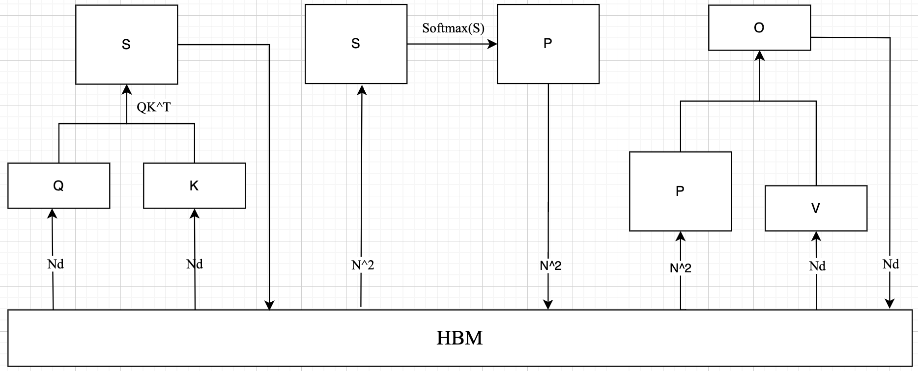
The problem is that for any non-trivial sequence length N (e.g., 2048, 4096, or more), the N x N matrix is far too large to fit in the fast on-chip SRAM of a GPU's Streaming Multiprocessor (SM).

For a concrete example, let's consider a single attention head for a sequence of length N = 4096 using fp16 (2 bytes per element). The intermediate attention matrix S would require:

$$4096\times 4096\times 2\text{ bytes}\approx 33.55\text{ MB}$$

Modern GPUs like the A100 have around 192 KB of L1/Shared Memory per SM. The 33.55 MB matrix is over 170 times larger than the available fast memory, leaving no choice but to store it in the much slower, off-chip HBM.

This forces the GPU into a memory-bound state, where the powerful compute units spend most of their time waiting for data to arrive from HBM, rather than performing actual calculations.

Profiling in Action: The Smoking Gun

Theory and diagrams are essential, but as a systems engineer, your conclusions must be backed by data. Let's see how ncu would reveal this bottleneck.

We'll revisit the "Reimplementing FlashAttention" article from our previous lesson. The author's initial "v1" implementation is a perfect stand-in for a naive, standard attention kernel. The profiling results are exactly what we would expect.

The analysis in the article is the crucial link between theory and practice. The profiler reports gigabytes of data being moved to and from DRAM (HBM), confirming that the operation is completely dominated by memory I/O.

When you see metrics like this in ncu, you can visualize the kernel's performance on a roofline chart.

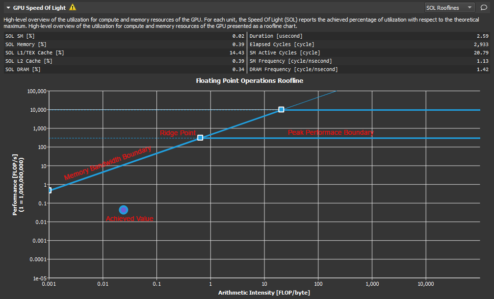
A kernel with low arithmetic intensity (few FLOPs per byte of data moved) and high memory traffic will land squarely in the memory-bound section of the roofline plot. This is a definitive sign that your optimization efforts should focus on reducing memory movement, not on optimizing the arithmetic operations themselves.

Quantifying the I/O Complexity

Let's formalize the I/O cost. As stated in Theorem 1 of the [Re] FlashAttention paper, the number of HBM accesses for standard attention is:

$\Theta (N^2+Nd)$

Let's break this down:

• Reads:
  • Read Q, K, V matrices from HBM: $O(Nd)$.
  • Read the intermediate (N,N) score matrix from HBM to compute the softmax: $O(N^2)$.
  • Read the (N,N) softmax output matrix P from HBM for the final multiplication: $O(N^2)$.
• Writes:
  • Write the intermediate (N,N) score matrix S to HBM: $O(N^2)$.
  • Write the (N,N) softmax output matrix P to HBM: $O(N^2)$.
  • Write the final output matrix O to HBM: $O(Nd)$.

The Nd terms correspond to the inputs and final output, which are unavoidable. The N^2 terms, however, are purely due to the materialization of the intermediate attention score matrix. As sequence length N grows, this quadratic term quickly dominates, making the HBM bandwidth the limiting factor for the entire operation. This is the memory-access bottleneck.

Conclusion

In this lesson, we moved from the mathematical definition of attention to a deep, hardware-level diagnosis of its performance. By combining theoretical analysis with the practical evidence from profiling tools, we have definitively identified the memory-access bottleneck in standard scaled dot-product attention.

Key Takeaways:

• The Bottleneck: Standard attention is memory-bound due to the need to read and write large O(N^2) intermediate matrices to and from slow off-chip HBM.
• The Evidence: Profiling tools like ncu make this bottleneck visible, reporting massive HBM/DRAM bandwidth usage (gigabytes of reads/writes) and showing the kernel's performance is limited by memory bandwidth on a roofline chart.
• The Cause: This is a direct consequence of implementing the attention equation literally. The intermediate (N, N) score matrix is too large for fast on-chip SRAM, forcing a dependency on HBM.
• The Complexity: The HBM access complexity is $\Theta(N^2 + Nd)$, with the quadratic term dominating as sequence length increases.

Preview of the Next Lesson:

Now that we have rigorously diagnosed the problem, we are ready to study the solution. In the next lesson, we will dive into FlashAttention. You will learn about the tiling and online softmax algorithm it uses to compute the exact same attention output without ever materializing the full N^2 matrix in HBM. This turns the memory-bound operation into a compute-bound one, unlocking massive speedups and making long-context models practical.