Tail Recursion with Accumulators

Hello! Welcome back to our module on "Recursion and Structural Thinking."

In our last lesson, we identified tail-recursive functions and saw how Tail-Call Optimization (TCO) makes them as memory-efficient as loops. We noted that this optimization is possible because there are no "pending operations" after the recursive call. We also had a glimpse of a pattern for achieving this using an "accumulator."

Today, we will formalize that pattern. The learning outcome for this lesson is to transform non-tail-recursive functions into tail-recursive form using the accumulator-passing style.

This is a fundamental skill in functional programming. It allows you to write elegant recursive solutions for problems that might otherwise seem to require loops, without sacrificing performance. We will cover:

1. A systematic method for this transformation.
2. Applications of the method to simple cases like factorial and list summation.
3. How to adapt the pattern for more complex recursions, like the Fibonacci sequence.
4. The direct relationship between this recursive style and imperative loops.

1. The Accumulator-Passing Style: A Systematic Method

The core idea is to stop storing pending operations implicitly on the call stack and instead pass the intermediate result explicitly as an argument to the function. This special argument is called an accumulator.

The transformation from a standard recursive function to a tail-recursive one using an accumulator generally follows a clear recipe.

To summarize and formalize the methodology:

1. Create a helper function: This new function will take the original arguments plus one or more new accumulator arguments. The main function becomes a simple "wrapper" that calls the helper with the initial value for the accumulator.
2. Define the new base case: In the helper function, the base case of the recursion no longer returns a fixed value (like 1 or 0). Instead, it returns the final value of the accumulator.
3. Redefine the recursive step: The "pending operation" from the original function (e.g., the multiplication in factorial) is now performed before the recursive call. The result is used to update the accumulator for the next call. This makes the recursive call the final action.

Let's see this recipe in action.

2. Application: Factorial and List Sum

Factorial

In the previous lesson, we saw the non-tail-recursive factorial: fact(n) = n * fact(n-1). The pending operation is the multiplication by n.

Let's apply our new methodology:

1. Helper function: We'll create fact_helper(n, acc). The main function fact(n) will call fact_helper(n, 1). Why 1? Because 1 is the identity element for multiplication; starting with it doesn't change the final product.
2. Base case: The original base case was fact(0) = 1. In our helper, when n is 0, the calculation is finished, and the result is in the accumulator. So, fact_helper(0, acc) returns acc.
3. Recursive step: The original step was n * fact(n-1). We now do the multiplication before the call: fact_helper(n-1, n * acc).

The following video walks through this exact transformation, providing a clear visual trace of how the accumulator builds up the result.

Sum of a List

Let's apply the same pattern to another common function: summing the elements of a list.

A simple, non-tail-recursive version is sum(lst) = head(lst) + sum(tail(lst)). The pending operation is the addition of head(lst).

Applying the methodology:

1. Helper function: sum_helper(lst, acc). The main function sum(lst) will call sum_helper(lst, 0). We use 0 as it's the identity element for addition.
2. Base case: The original base case was sum([]) = 0. Our helper's base case is sum_helper([], acc), which returns acc.
3. Recursive step: The new step is sum_helper(tail(lst), head(lst) + acc).

The following resource shows this transformation in both Python and Haskell. It also includes an important note about Python's design philosophy, which is relevant to your goals.

3. A More Complex Case: The Fibonacci Sequence

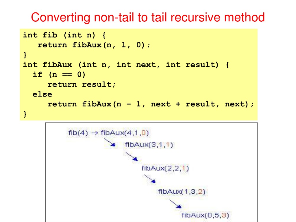
The standard recursive definition fib(n) = fib(n-1) + fib(n-2) is notoriously inefficient. It's also not tail-recursive because the final operation is +. Furthermore, it has two recursive calls, not one.

How can we apply the accumulator pattern here? We can't just accumulate the sum. We need to keep track of the two previous numbers in the sequence to compute the next one. This means we need two accumulators.

The strategy is to use two accumulators that represent a "sliding window" of the two latest Fibonacci numbers, say current and next.

1. Helper function: fib_helper(n, current, next).
2. Initial call: To compute fib(n), we start the process with the 0th and 1st Fibonacci numbers: fib_helper(n, 0, 1).
3. Base case: When the counter n reaches 0, the current accumulator holds our desired result. So, fib_helper(0, current, next) returns current.
4. Recursive step: In each step, we decrement n and slide the window: the old next becomes the new current, and current + next becomes the new next. The call is fib_helper(n-1, next, current + next).

This is a clever and powerful extension of the accumulator pattern. The Computerphile video explains this "sliding window" concept very intuitively.

For a static reference, this image provides a concise summary of the code and an execution trace.

4. The Connection to Iteration

At this point, you might notice a strong similarity between the tail-recursive functions we've built and simple imperative loops. This is not a coincidence. Tail recursion is the functional paradigm's equivalent of iteration.

• The helper function's arguments (including accumulators) correspond to the state variables of a loop.
• The initial call to the helper function initializes these state variables.
• The base case of the recursion is the loop's termination condition.
• The recursive call is the next iteration of the loop, updating the state variables.

This equivalence is so direct that you can mechanically translate one to the other. Given your proficiency in Python, this connection should be very clear.

This insight is crucial. It shows that by preferring recursion, functional languages don't lose the power of iteration; they just express it differently. TCO is the mechanism that ensures this expressive power doesn't come with a performance penalty.

Conclusion

Today we've established a powerful and systematic technique for converting non-tail-recursive functions into their efficient, tail-recursive counterparts.

Key Takeaways:

• Accumulator-passing style is the primary method for this transformation. It involves a helper function that carries intermediate results in an extra argument (the accumulator).
• The initial value of the accumulator is typically the identity element of the pending operation (e.g., 0 for addition, 1 for multiplication).
• For more complex state dependencies, like in Fibonacci, multiple accumulators can be used to pass the required state through the recursive calls.
• Tail recursion is structurally equivalent to imperative iteration. A tail-recursive function can be mechanically translated into a while loop, and vice-versa.

Next Lesson Preview:

Now that we understand that tail recursion and iteration are two sides of the same coin, we are ready to explore the design trade-offs between them. In our next lesson, we will compare the recursion-first philosophy of languages like Haskell with the iteration-first philosophy of languages like Python, analyzing how these different defaults influence problem-solving strategies and code style.