RLC Circuit Second-Order ODEs

Hello! Welcome to the next lesson in our radioelectronics course.

In our previous lessons, we thoroughly analyzed first-order circuits (RC and RL), which contain a single energy-storage element. We saw that their behavior is described by first-order ODEs, leading to exponential responses. Now, we will explore what happens when we combine all three passive components—a resistor, a capacitor, and an inductor—into one circuit.

Introduction

Approximate time to complete: 45 minutes.

This lesson focuses on the learning outcome: Deriving the Second-Order ODE for Series and Parallel RLC Circuits. We will use the fundamental circuit laws you're familiar with to build the mathematical models that govern these more complex circuits.

Recap from previous lessons:

• KVL & KCL: The foundational laws for analyzing voltages in a loop and currents at a node.
• Component V-I Relationships:
  • Resistor: $v=iR$
  • Inductor: $v=L\frac{di}{dt}$
  • Capacitor: $i=C\frac{dv}{dt}$ or $v=\frac{1}{C}\int i(t)dt$
• First-order circuits, with one energy storage element, are described by first-order ODEs.

Today, we'll see how adding a second, independent energy storage element elevates the system's complexity, requiring a second-order ODE to describe it.

---

1. What Makes a Circuit "Second-Order"?

A first-order system, like an RC or RL circuit, can only store and dissipate energy. The capacitor or inductor charges or discharges, and the response always moves in one direction towards its final value (an exponential curve).

A second-order system has two independent energy storage elements. In an RLC circuit, the inductor stores energy in a magnetic field, and the capacitor stores it in an electric field. This creates a new dynamic: the two elements can exchange energy back and forth.

This energy exchange is what allows for oscillation—a behavior impossible in first-order circuits.

Please watch the first part of this video for an excellent analogy and explanation of what makes a system second-order.

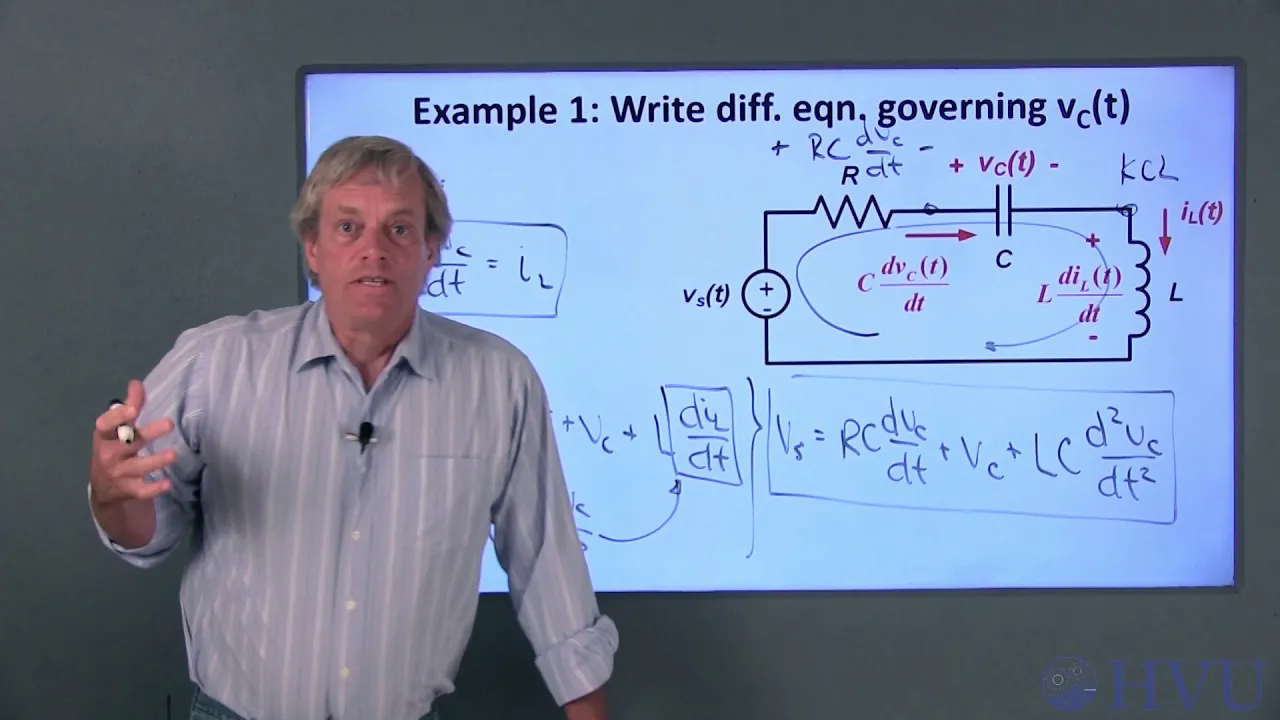
Focus on the segment from 00:00:20 to 00:03:10. The analogy of a swingset, where kinetic and potential energy are traded, is a perfect mechanical parallel to the electrical and magnetic energy exchange in an RLC circuit. This oscillation is a fundamental concept in radio tuners, filters, and oscillators.

2. A Systematic Approach to Derivation

Deriving these ODEs is not a random process. We can follow a clear, repeatable strategy that works for any circuit, no matter how complex. This approach leverages the skills you already have.

The same video outlines a robust four-step method. Watch the next segment from 00:03:10 to 00:05:41 for a summary of this process.

Here is a summary of the steps:

1. Label Energy Storage Variables: Identify the capacitor voltage ($v_C$) and inductor current ($i_L$) as your primary variables.
2. Define Other Quantities: Use the V-I relationships to express other circuit quantities (like capacitor current or inductor voltage) in terms of $v_C$ and $i_L$.
3. Apply KVL/KCL: Write loop (KVL) and node (KCL) equations until you have as many equations as you have unknown variables.
4. Combine and Eliminate: Use algebraic substitution and differentiation to combine your equations and eliminate all variables except the one you want to solve for. The result will be a single second-order ODE.

With this framework in mind, let's derive the equations for our two main RLC configurations.

---

3. The Series RLC Circuit

Let's start with a source-free series RLC circuit (also known as the "natural response"). This is the simplest case and directly leads to the homogeneous ODE we will solve in the next lesson.

Here, the resistor, inductor, and capacitor are all in a single loop. Applying Kirchhoff's Voltage Law (KVL) is the most direct approach. The sum of the voltage drops across each component must be zero.

The following video provides a concise and clear derivation. Please watch this segment, which walks through applying KVL and then differentiating the resulting equation to arrive at the final second-order ODE.

Watch the derivation for the series circuit from 00:06:54 to 00:10:56.

Let's break down the steps shown in the video:

1. Apply KVL: We sum the voltages around the loop:
   $v_R+v_L+v_C=0$

2. Express in terms of current $i(t)$: The common variable in a series circuit is the current $i$.
   $Ri(t)+L\frac{di}{dt}+\frac{1}{C}{\int }_0^{t}i(\tau )d\tau +v_C(0)=0$
   This gives us an integro-differential equation—it contains both an integral and a derivative.

3. Differentiate to Eliminate the Integral: To convert this into a pure ODE, we take the derivative of the entire equation with respect to time:
   $R\frac{di}{dt}+L\frac{d^{2}i}{d{t}^2}+\frac{1}{C}i(t)=0$

4. Standard Form: Finally, we rearrange the terms by descending order of derivative and divide by $L$ to isolate the highest-order term. This gives us the standard form of the second-order homogeneous ODE for a series RLC circuit:
   $\frac{d^{2}i}{d{t}^2}+\frac{R}{L}\frac{di}{dt}+\frac{1}{LC}i=0$

---

4. The Parallel RLC Circuit

Now, let's analyze the source-free parallel RLC circuit. In this configuration, all three components share the same two nodes. Here, applying Kirchhoff's Current Law (KCL) at one of the nodes is the most logical starting point. The sum of the currents leaving the node must be zero.

The same video also provides an excellent walkthrough for the parallel case. Please watch this segment carefully.

Watch the derivation for the parallel circuit from 00:02:13 to 00:06:54.

Let's summarize the key steps for the parallel circuit:

1. Apply KCL: We sum the currents leaving the top node:
   $i_R+i_L+i_C=0$

2. Express in terms of voltage $v(t)$: The common variable across parallel components is the voltage $v$.
   $\frac{v(t)}{R}+\left(\frac{1}{L}{\int }_0^{t}v(\tau )d\tau +i_L(0)\right)+C\frac{dv}{dt}=0$
   Again, we have an integro-differential equation.

3. Differentiate to Eliminate the Integral: As before, we differentiate the entire equation with respect to time:
   $\frac{1}{R}\frac{dv}{dt}+\frac{1}{L}v(t)+C\frac{d^{2}v}{d{t}^2}=0$

4. Standard Form: We rearrange and divide by $C$ to get the standard form of the second-order homogeneous ODE for a parallel RLC circuit:
   $\frac{d^{2}v}{d{t}^2}+\frac{1}{RC}\frac{dv}{dt}+\frac{1}{LC}v=0$

---

5. The General Form and What It Means

Take a close look at the two equations we've just derived:

• Series: $\frac{d^{2}i}{d{t}^2}+\frac{R}{L}\frac{di}{dt}+\frac{1}{LC}i=0$
• Parallel: $\frac{d^{2}v}{d{t}^2}+\frac{1}{RC}\frac{dv}{dt}+\frac{1}{LC}v=0$

Notice a crucial pattern? Both equations fit the same general mathematical structure:

$\frac{d^{2}x}{d{t}^2}+2\alpha \frac{dx}{dt}+{\omega }_0^{2}x=0$

This is the standard form for a homogeneous second-order linear ordinary differential equation with constant coefficients. In this form:

• ${\omega }_0$ is the undamped resonant frequency. It's the natural frequency at which the circuit wants to oscillate if there were no resistance ($R=0$). It is the same for both series and parallel configurations:
  ${\omega }_0=\frac{1}{\sqrt{LC}}$
• $\alpha$ is the damping factor or neper frequency. It determines how quickly the oscillations die out due to energy dissipation in the resistor. Its form depends on the circuit topology:
  • For a series RLC circuit: $\alpha =\frac{R}{2L}$
  • For a parallel RLC circuit: $\alpha =\frac{1}{2RC}$

The relationship between $\alpha$ and ${\omega }_0$ will dictate the exact nature of the circuit's response, a topic we will explore in depth in our next lesson.

Conclusion

In this lesson, we made the critical leap from first-order to second-order systems. We established that RLC circuits are second-order because their two energy storage elements (L and C) can exchange energy, allowing for oscillation.

Key Takeaways:

• RLC circuits are modeled by second-order ordinary differential equations.
• The derivation process involves applying KVL (for series) or KCL (for parallel) and then differentiating the resulting integro-differential equation.
• The ODEs for both series and parallel circuits can be expressed in the general form $\frac{d^{2}x}{d{t}^2}+2\alpha \frac{dx}{dt}+{\omega }_0^{2}x=0$.
• The damping factor ($\alpha$) and the resonant frequency (${\omega }_0$) are crucial parameters determined by the R, L, and C values that define the circuit's behavior.

Preview of the Next Lesson:

We have successfully derived the governing equations. The next logical step is to solve them. In the upcoming lesson, "Solving the Homogeneous Second-Order RLC ODE," we will find the solution to this general ODE. We will discover that the form of the solution changes dramatically based on whether $\alpha$ is greater than, equal to, or less than ${\omega }_0$, leading to the three fundamental responses: overdamped, critically damped, and underdamped. This is where the rich behavior of RLC circuits truly begins to unfold.