FastSpeech 2: Non-Autoregressive TTS with Variance Adaptor

Hello! Welcome to your next lesson on Text-to-Speech architectures.

In our last session, we took a deep dive into Tacotron 2, a powerful autoregressive model. We saw how its sequential, frame-by-frame generation process, guided by location-sensitive attention, produces high-quality, natural-sounding speech. However, we also noted its main drawback: the autoregressive nature makes inference inherently slow, as each new frame depends on the previously generated one.

Today, we will explore a groundbreaking model that directly tackles this speed limitation: FastSpeech 2. Our learning outcome is to describe the FastSpeech 2 architecture, highlighting its non-autoregressive design and variance adaptor module. We will see how it achieves massive speed-ups by generating the entire mel-spectrogram in parallel, and how it solves the challenges this new paradigm introduces.

By the end of this lesson, you'll understand the architectural shift from sequential to parallel TTS and appreciate the clever design of the components that make it possible.

1. The Leap to Parallel Generation: Non-Autoregressive TTS

The core difference between models like Tacotron 2 and FastSpeech 2 lies in their fundamental generation strategy: autoregressive vs. non-autoregressive.

As the diagram shows, autoregressive models are sequential. This dependency chain is great for modeling complex distributions but creates a bottleneck at inference time. Non-autoregressive models break this chain, generating all output steps simultaneously. This leads to a dramatic increase in synthesis speed.

However, this parallelism comes with a significant challenge, known as the one-to-many mapping problem. A single text sentence can be spoken in many different ways, with variations in speed, pitch, and emphasis.

• Tacotron 2 handles this implicitly. By conditioning on the previous mel-spectrogram frame, it learns to continue a specific prosodic contour.
• FastSpeech 2, lacking this sequential context, must be explicitly given information about the desired speech variation. Without it, the model would be forced to average all possible variations, resulting in bland, unnatural speech.

Let's watch a short clip that introduces the motivation for parallel generation and names FastSpeech 2 as a key example.

The first version of FastSpeech attempted to solve the one-to-many problem using a complex "teacher-student" training pipeline. It relied on a trained Tacotron 2 model to provide phoneme duration alignments and to "distill" knowledge into the simpler, faster model. FastSpeech 2 improves upon this by removing the dependency on a teacher model, resulting in a simpler training process and often higher quality.

2. FastSpeech 2: Architectural Overview

FastSpeech 2 is a fully feed-forward network based on the Transformer architecture. It takes a sequence of phonemes as input and generates a corresponding mel-spectrogram in a single pass.

Let's start by studying the original paper's introduction to the model.

As the paper describes, FastSpeech 2 has three main components, which we can see in the overall architecture diagram.

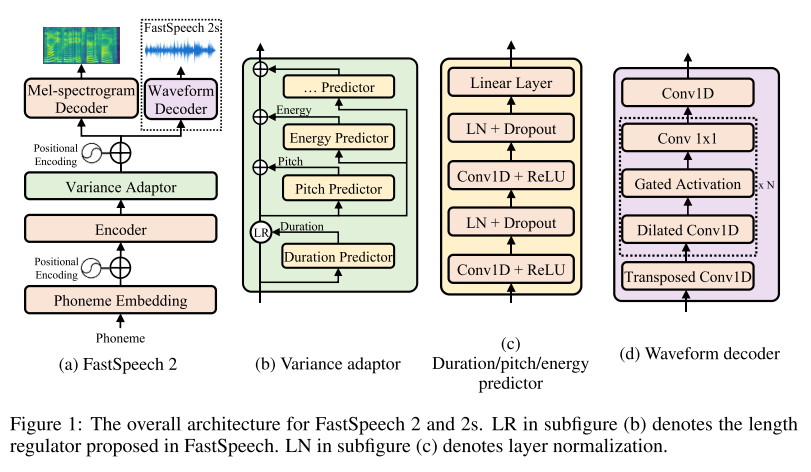
Let's break down the data flow:

1. A Phoneme Encoder converts the input phoneme sequence into a sequence of hidden representations.
2. The Variance Adaptor, the core of the model, injects speech variation information (duration, pitch, energy) into the hidden sequence.
3. A Mel-Spectrogram Decoder takes the adapted hidden sequence and converts it into a mel-spectrogram.

Crucially, every component in this pipeline is non-autoregressive. Let's examine each part in detail, starting with the most important innovation.

3. The Heart of the Model: The Variance Adaptor

The Variance Adaptor is FastSpeech 2's solution to the one-to-many mapping problem. Instead of letting the model figure out prosody implicitly, the Variance Adaptor explicitly models the main sources of variation in speech and provides them as conditional information to the decoder.

Let's dive into the details of this module.

The Variance Adaptor consists of several predictor modules and a length regulator. Let's analyze each one.

3.1 Duration Predictor and Length Regulator

This is the mechanism that replaces Tacotron 2's attention. Instead of learning to align text and speech at each step, FastSpeech 2 explicitly predicts the duration of each phoneme.

• Duration Predictor: A simple 2-layer 1D CNN that takes the encoder's hidden states and predicts a single duration value (in a log scale) for each phoneme. This value represents how many mel-spectrogram frames the phoneme should last.
• Training: During training, the ground-truth durations are obtained using an external tool called a forced aligner (e.g., Montreal Forced Aligner), which aligns the input text with the audio data at the phoneme level. The predictor is trained with an MSE loss to match these ground-truth durations.
• Length Regulator (LR): This is not a neural network but a simple operation. It takes the sequence of hidden states from the encoder and expands it based on the predicted durations. For example, if the phoneme /ae/ has a predicted duration of 5, the Length Regulator repeats the hidden state for /ae/ five times. This expands the phoneme-level sequence to match the length of the frame-level mel-spectrogram, solving the length mismatch problem.

This duration prediction and expansion mechanism is the key that unlocks parallel generation.

3.2 Pitch and Energy Predictors

Duration alone isn't enough to capture the richness of speech. Pitch (related to intonation) and energy (related to volume) are also crucial.

• Pitch Predictor: This module predicts the fundamental frequency (F0) contour on a frame-by-frame basis.

  • Modeling Pitch: The FastSpeech 2 paper notes that pitch can be highly variable and difficult to predict directly. To handle this, it uses a more sophisticated approach. The pitch contour is first decomposed into a pitch spectrogram using a Continuous Wavelet Transform (CWT). The predictor is trained to predict this spectrogram, which is then converted back to a pitch contour during inference via an Inverse CWT. This is a great example of applying signal processing concepts to improve a deep learning model.
  • Input to Decoder: The predicted pitch value for each frame is quantized, converted to an embedding vector, and added to the expanded hidden sequence.

• Energy Predictor: This module predicts the energy for each frame, which corresponds to the magnitude (volume) of the speech.

  • How it works: It predicts the L2-norm of the amplitude of each STFT frame. Like the pitch, the predicted energy value is quantized, embedded, and added to the hidden sequence.

By the time the hidden sequence leaves the Variance Adaptor, it has been expanded to the correct length and enriched with explicit information about the duration, pitch, and energy of the target speech. This gives the decoder all the information it needs to generate a specific speech variation in parallel. A major benefit is that during inference, we can manually alter the outputs of these predictors to control the speed, pitch, and volume of the synthesized voice.

4. Encoder and Decoder: Feed-Forward Transformers

With the core complexity handled by the Variance Adaptor, the encoder and decoder architectures are relatively straightforward. Both are composed of a stack of Feed-Forward Transformer (FFT) blocks.

An FFT block is a slight modification of the standard Transformer block you're familiar with from sequence modeling.

• Structure: It consists of a multi-head self-attention layer followed by a 2-layer 1D CNN, with residual connections and layer normalization around each sub-layer.
• Rationale for 1D CNNs: The original Transformer uses a fully-connected feed-forward network. The FastSpeech authors replaced this with 1D CNNs because in sequences like phonemes or spectrograms, adjacent elements are highly correlated. CNNs are excellent at capturing these local patterns, making them a better fit for this task.

Encoder:
The encoder's job is to create a contextual representation of the input phonemes. It's a stack of FFT blocks that processes the sequence of phoneme embeddings (plus positional encodings) and outputs a sequence of contextual hidden states.

Decoder:
The decoder is architecturally identical to the encoder. It takes the output from the Variance Adaptor—the expanded and variation-enriched hidden sequence—and passes it through its own stack of FFT blocks. The final output is projected by a linear layer to produce the 80-channel mel-spectrogram for the entire utterance at once.

Conclusion

In this lesson, we have dissected the architecture of FastSpeech 2, a pioneering non-autoregressive TTS model. We've contrasted its parallel approach with the sequential nature of Tacotron 2 and examined the key components that enable its speed and quality.

Key Takeaways:

• Non-Autoregressive Design: FastSpeech 2 generates the entire mel-spectrogram in parallel, making inference significantly faster than autoregressive models like Tacotron 2.
• The One-to-Many Problem: The main challenge for non-autoregressive TTS is resolving the ambiguity of speech variations.
• Variance Adaptor: This is FastSpeech 2's solution. It explicitly models and predicts key speech variations:
  • Duration: A predictor determines the length of each phoneme, and a Length Regulator expands the encoder outputs accordingly, replacing the need for an attention mechanism.
  • Pitch & Energy: Predictors for pitch (F0) and energy (volume) provide frame-level prosodic information.
• Controllability: Because duration, pitch, and energy are explicitly predicted, they can be manually adjusted at inference time to control the synthesized speech.
• Transformer-Based: The encoder and decoder are built from Feed-Forward Transformer (FFT) blocks, which use self-attention to capture global dependencies and 1D CNNs to model local patterns.

Preview of the Next Lesson:

We have now explored two landmark architectures: the autoregressive Tacotron 2 and the non-autoregressive FastSpeech 2. In the next lesson, we will directly compare these two paradigms. We will analyze their trade-offs in terms of synthesis quality, speed, robustness, controllability, and training complexity to understand when and why you might choose one over the other.