Calculating AMM Spot Price, Price Impact, and Slippage

Welcome to the decentralized-exchange module. In the previous module, you learned to map a DeFi protocol’s actors, assets, controls, dependencies, and risk bearers. We now apply that discipline to an automated market maker, or AMM: a smart contract that lets traders swap against pooled assets rather than matched orders.

This lesson focuses on the simplest and most influential AMM design, the constant-product market maker. You will calculate:

• the pool’s spot price;
• a swap’s execution price and price impact;
• slippage between the quote you expected and the amount that actually executes.

The calculations are based on a two-token, full-range constant-product pool, the model associated with Uniswap V2. Later lessons will examine liquidity-provider exposure and concentrated liquidity; for now, stay focused on the trader’s quote and execution.

---

A pool is the counterparty to the trade

In an order-book exchange, a trader usually trades against other traders’ limit orders. In a constant-product AMM, a trader trades against a pool holding two assets.

Let:

• $x$ be the reserve of token $X$;
• $y$ be the reserve of token $Y$;
• $k$ be their product.

The pool follows the invariant:

$$xy=k$$

A trader who sells $X$ to receive $Y$ increases the pool’s $X$ reserve and removes some $Y$ reserve. The amount of $Y$ paid out is constrained by the requirement that the pool remain on its pricing curve.

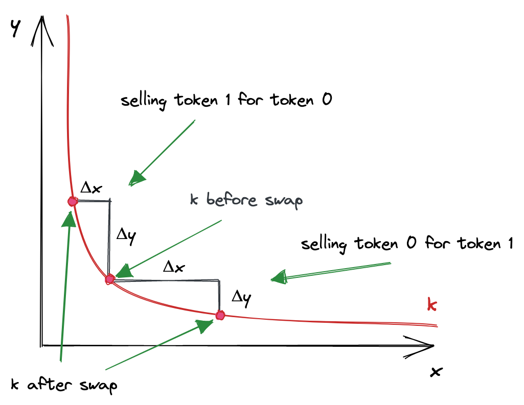
The essential economic feature is straightforward: the pool always offers a price, but that price worsens as a trade becomes large relative to its reserves. The pool cannot be drained at a finite price because acquiring the final units of an asset would require an increasingly extreme amount of the other asset.

---

Define the price before calculating it

Suppose $X$ is ETH and $Y$ is USDC. If a pool contains $10$ ETH and $20,000$ USDC, then the pool’s initial state is:

$$x=10$$ $$y=20,000$$ $$k=10\times 20,000=200,000$$

The spot price of $X$ in units of $Y$ is the reserve ratio:

$$p_0=\frac{y}{x}$$

For the ETH/USDC example:

$$p_0=\frac{20,000}{10}=2,000$$

So the initial spot price is $2,000$ USDC per ETH.

This is a marginal price: it describes the rate for an infinitesimally small trade. It is not generally the rate a trader receives for a finite trade.

The reciprocal is the spot price of $Y$ in $X$:

$$p_0^Y=\frac{x}{y}$$

In the example:

$$p_0^Y=\frac{10}{20,000}=0.0005$$

So $1$ USDC is worth $0.0005$ ETH at the pool’s initial marginal price.

The geometric interpretation

The constant-product curve can be written as:

$$y=\frac{k}{x}$$

Its slope is negative because adding $X$ to the pool requires $Y$ to leave it. The magnitude of the slope at a point is:

$$\left|\frac{dy}{dx}\right|=\frac{y}{x}$$

That is why the reserve ratio gives the spot price. The price is the tangent to the curve at the current pool state. A real swap, by contrast, travels between two points on the curve, so it has an average execution price rather than a single marginal price.

---

Calculate swap output and execution price

Assume first that the pool charges no trading fee. A trader sends $\Delta x$ units of $X$ into the pool and receives $\Delta y$ units of $Y$.

The pool begins with:

$$xy=k$$

After the swap, its reserves are:

$$x_1=x+\Delta x$$ $$y_1=y-\Delta y$$

The invariant requires:

$$(x+\Delta x)(y-\Delta y)=xy$$

Solving for output gives the central constant-product swap formula:

$$\Delta y=\frac{y\Delta x}{x+\Delta x}$$

The trader’s average execution price, expressed as units of $Y$ received for each unit of $X$ sold, is:

$$p_{\text{exec}}=\frac{\Delta y}{\Delta x}$$

Substituting the output formula gives:

$$p_{\text{exec}}=\frac{y}{x+\Delta x}$$

Compare this with the initial spot price:

$$p_0=\frac{y}{x}$$

Because $x+\Delta x$ is greater than $x$, the execution price is lower than the initial spot price when selling $X$. You receive fewer units of $Y$ per unit of $X$ than a simple spot-price multiplication would suggest.

---

Worked example: selling ETH for USDC

Return to the pool with $10$ ETH and $20,000$ USDC. A trader sells $1$ ETH to the pool.

The trader might naively expect:

$$1\times 2,000=2,000\text{ USDC}$$

But $2,000$ USDC is only the initial spot-price estimate. The actual fee-free output is:

$$\Delta y=\frac{20,000\times 1}{10+1}$$ $$\Delta y=1,818.18\text{ USDC}$$

The pool’s final reserves are:

$$x_1=10+1=11\text{ ETH}$$ $$y_1=20,000-1,818.18=18,181.82\text{ USDC}$$

Check the invariant:

$$11\times 18,181.82\approx 200,000$$

The average execution price is:

$$p_{\text{exec}}=\frac{1,818.18}{1}$$ $$p_{\text{exec}}=1,818.18\text{ USDC per ETH}$$

The trader sold ETH into the pool, so ETH became more abundant in that pool and USDC became scarcer. Accordingly, ETH’s post-swap spot price in USDC falls:

$$p_1=\frac{18,181.82}{11}$$ $$p_1=1,652.89\text{ USDC per ETH}$$

There are therefore three distinct prices worth keeping separate:

Price	Meaning	ETH/USDC example
Initial spot price	Marginal rate before the trade	$2,000$ USDC per ETH
Execution price	Average rate across the trader’s finite swap	$1,818.18$ USDC per ETH
Final spot price	Marginal rate after the trade	$1,652.89$ USDC per ETH

The execution price lies between the initial and final spot prices because it is an average across the movement along the curve.

---

Price impact: the cost caused by your own trade

Price impact is the deterioration in price caused by the trade itself moving the pool along its curve. It is not a network fee, and it is not necessarily evidence that anything unexpected happened.

For a trade that sells $X$ for $Y$, define curve price impact as the shortfall of the execution price relative to the pre-trade spot price:

$$\text{Price impact}=1-\frac{p_{\text{exec}}}{p_0}$$

Using the constant-product formulas:

$$\text{Price impact}=1-\frac{y/(x+\Delta x)}{y/x}$$ $$\text{Price impact}=\frac{\Delta x}{x+\Delta x}$$

In the example:

$$\text{Price impact}=\frac{1}{10+1}=9.09\%$$

The trader receives $9.09\%$ less USDC than the initial spot-price estimate. Equivalently:

$$2,000-1,818.18=181.82\text{ USDC}$$

This is the curve-induced shortfall for the trader’s $1$ ETH trade.

Trade size relative to liquidity matters

A useful result is that the absolute dollar size of a trade is not enough to judge price impact. What matters is its size relative to the input reserve.

In the same pool:

ETH input	Fraction of ETH reserve	Fee-free price impact
$0.01$ ETH	$0.1\%$	about $0.10\%$
$0.10$ ETH	$1\%$	about $0.99\%$
$1.00$ ETH	$10\%$	$9.09\%$
$5.00$ ETH	$50\%$	$33.33\%$

A $1$ ETH swap is very large for a pool with only $10$ ETH, but potentially negligible for a pool holding tens of thousands of ETH. This is why deeper liquidity improves execution quality.

Do not confuse execution-price impact with post-trade spot movement

Another valid but different calculation compares the post-trade marginal price with the initial marginal price:

$$1-\frac{p_1}{p_0}=1-{\left(\frac{x}{x+\Delta x}\right)}^2$$

For the $1$ ETH trade:

$$1-\frac{1,652.89}{2,000}=17.36\%$$

This $17.36\%$ figure is the movement in the pool’s marginal ETH price from before to after the trade. It is not the trader’s average price impact, which was $9.09\%$.

When reviewing a DEX interface, dashboard, or research note, always ask which definition it uses:

• execution price versus initial spot price; or
• final spot price versus initial spot price.

Both may be described informally as “price impact,” but they measure different things.

---

Incorporate a trading fee

Most AMMs charge a fee. Let:

$$f=\text{fee rate}$$ $$r=1-f$$

For a $0.3\%$ fee:

$$f=0.003$$ $$r=0.997$$

If the trader sends $\Delta x$ into the pool, the amount used in the pricing calculation is:

$$\Delta x_{\text{effective}}=r\Delta x$$

The fee-adjusted output formula is:

$$\Delta y_{\text{fee}}=\frac{yr\Delta x}{x+r\Delta x}$$

For the same $10$ ETH and $20,000$ USDC pool, selling $1$ ETH produces:

$$\Delta y_{\text{fee}}=\frac{20,000\times 0.997\times 1}{10+0.997\times 1}$$ $$\Delta y_{\text{fee}}\approx 1,813.22\text{ USDC}$$

The fee-inclusive execution price is:

$$p_{\text{exec, fee}}=\frac{1,813.22}{1}=1,813.22\text{ USDC per ETH}$$

Relative to the initial spot price, the total quoted shortfall is:

$$1-\frac{1,813.22}{2,000}=9.34\%$$

That $9.34\%$ combines two distinct effects:

1. the AMM curve worsens the price for a large trade;
2. the protocol deducts a trading fee.

Do not simply add $9.09\%$ and $0.3\%$. The fee changes the effective amount moving along the curve, so the exact fee-inclusive calculation should use the swap formula.

A practical detail about $k$ and fees

Without fees, the post-swap reserves satisfy:

$$x_1{y}_1=k$$

In many fee-charging AMMs, the fee remains in the pool. The output is calculated using $r\Delta x$, but the full input amount is retained in the actual reserve. Therefore, the observed reserve product after the trade can increase slightly:

$$(x+\Delta x)(y-\Delta y_{\text{fee}})>k$$

That increase represents fee value retained for liquidity providers, subject to any protocol-level fee arrangement. For trade-quote calculations, use the effective-input formula; do not assume that the raw post-swap reserve product will be exactly unchanged in a fee-charging implementation.

---

Slippage: the difference between quote and execution

In common trading usage, slippage is the difference between the amount you expected when submitting a transaction and the amount actually received when it executes.

Suppose the AMM quote when you sign the transaction is:

$$Q=1,813.22\text{ USDC}$$

If the transaction later executes and you receive $A$ USDC, realized adverse slippage is:

$$\text{Slippage}=1-\frac{A}{Q}$$

This definition distinguishes slippage from the known, deterministic price impact already included in the quote.

Why actual output can differ from the quote

Between transaction submission and inclusion on-chain, the pool state can change. Common causes include:

• other traders swapping in the same pool;
• arbitrage transactions updating the pool toward an external market price;
• delayed inclusion during congestion;
• transaction ordering or maximal extractable value.

Consider the earlier example without fees so the arithmetic remains transparent. Your quote for selling $1$ ETH is:

$$Q=1,818.18\text{ USDC}$$

Before your transaction executes, another trader sells $0.5$ ETH into the same pool. That first trade changes the reserves to approximately:

$$x=10.5\text{ ETH}$$ $$y=19,047.62\text{ USDC}$$

Your $1$ ETH transaction now executes against this less favorable state:

$$A=\frac{19,047.62\times 1}{10.5+1}$$ $$A\approx 1,656.32\text{ USDC}$$

Your realized slippage relative to the original quote is:

$$1-\frac{1,656.32}{1,818.18}\approx 8.90\%$$

Your original quote already reflected your own $9.09\%$ price impact. The additional $8.90\%$ is caused by the intervening trade changing the pool state.

Slippage tolerance is a minimum-output condition

A DEX usually lets a trader specify a slippage tolerance. For an exact-input swap, it translates to a minimum acceptable output:

$$\text{minimum output}=Q(1-s)$$

where $s$ is the tolerance.

If the fee-inclusive quote is $1,813.22$ USDC and you set $s=1\%$, then:

$$\text{minimum output}=1,813.22(1-0.01)$$ $$\text{minimum output}\approx 1,795.09\text{ USDC}$$

If the contract cannot provide at least $1,795.09$ USDC, the transaction reverts rather than executing at a worse rate. The user will generally still pay for the gas consumed by the failed transaction.

A loose tolerance reduces the chance of a failed trade but accepts a wider range of outcomes. A very tight tolerance limits adverse execution but may cause ordinary trades to fail in volatile or congested conditions. It is an execution constraint, not a guarantee of fair market price.

---

A repeatable calculation workflow

For a constant-product pool, use this process before trusting a displayed quote.

1. Set the direction and units.
   Define input token $X$, output token $Y$, and ensure that $x$, $y$, and $\Delta x$ all use consistent units.

2. Calculate the initial spot price.

   $$p_0=\frac{y}{x}$$

   This is the marginal price of $X$ in units of $Y$.

3. Calculate effective input if there is a fee.

   $$\Delta x_{\text{effective}}=(1-f)\Delta x$$

4. Calculate expected output.

   $$\Delta y=\frac{y\Delta x_{\text{effective}}}{x+\Delta x_{\text{effective}}}$$

5. Calculate the execution price.

   $$p_{\text{exec}}=\frac{\Delta y}{\Delta x}$$

6. Report price impact with a stated convention.
   For the fee-free curve-only convention:

   $$\text{Price impact}=1-\frac{p_{\text{exec}}}{p_0}$$

   For a fee-charging pool, distinguish curve-only impact from the total quote shortfall.

7. Set or evaluate minimum output.

   $$\text{minimum output}=Q(1-s)$$

8. After execution, compare actual output with the quote.

   $$\text{Realized slippage}=1-\frac{A}{Q}$$

Decimal-normalization warning

On-chain reserve values are usually stored in smallest units, not in human-readable token amounts. ETH has $18$ decimals and USDC commonly has $6$. If using raw contract balances, normalize them first:

$$x_{\text{human}}=\frac{x_{\text{raw}}}{10^{d_x}}$$ $$y_{\text{human}}=\frac{y_{\text{raw}}}{10^{d_y}}$$

Then calculate:

$$p_0=\frac{y_{\text{human}}}{x_{\text{human}}}$$

Failing to account for decimal differences can produce a price that is wrong by factors of millions or trillions even when the AMM formula itself is correct.

---

Key takeaways

A constant-product AMM prices trades from pool reserves rather than an order book:

$$xy=k$$

• The initial spot price of $X$ in $Y$ is $y/x$.
• A finite swap has an average execution price, not the initial spot price.
• For a fee-free exact-input swap, output is:

$$\Delta y=\frac{y\Delta x}{x+\Delta x}$$

• Price impact increases with trade size relative to the pool’s input reserve.
• Trading fees reduce output further and must be separated conceptually from curve-induced price impact.
• Slippage is the gap between your quoted output and actual output after the pool state changes before execution.
• A slippage tolerance sets a minimum acceptable output; it does not remove market, timing, or transaction-ordering risk.

Next, you will shift from the trader’s perspective to the liquidity provider’s: how the pool’s asset composition changes as relative prices move, and why fee income does not by itself determine an LP’s return.