Deriving Time-Complexity Targets from Input Constraints

Hello. This first module builds a habit that separates many accepted solutions from elegant time-limit failures: reading constraints as design requirements, not as decoration. Before selecting a data structure or proving a greedy idea, you need a realistic ceiling on the work your program may perform.

In this lesson, you will turn a time limit, per-test bounds, and aggregate bounds such as “the sum of $n$ over all test cases is at most $S$” into a feasible complexity target. The important refinement is that a total-size bound makes linear work aggregate cleanly, but it does not automatically make every nonlinear algorithm safe.

---

Constraints are an algorithm-selection filter

A problem statement gives you an input-size envelope. Your first task is to estimate which algorithm families can fit inside it.

At a deliberately rough level, a C++ solution under a one-second limit may handle on the order of $10^7$ to $10^8$ very simple operations. This is not a law:

• Integer additions and array accesses are cheap.
• Division, modulo, hashing, balanced-tree operations, allocation, recursion overhead, and heavy object use cost more.
• Input parsing and output can matter on very large instances.
• The judge machine and language affect the constant factor.

So treat an operation budget as a conservative engineering estimate, not as a proof of acceptance. For a typical Codeforces solution, your goal is not to land precisely on the estimated limit; it is to leave enough margin for constants, hidden test structure, and implementation overhead.

The point of the familiar Big-O growth chart is not that one curve is morally “good” and another “bad.” It is that the size of $n$ changes the meaning of a complexity class. An $O(n^2)$ method may be ideal for $n\le 2000$, yet impossible for $n\le 2\cdot 10^5$.

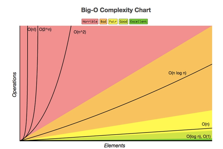
A useful first-pass calibration for simple C++ implementations is:

Largest relevant size	Often plausible	Usually suspicious
$n\le 20$	$O(2^n\cdot \mathrm{poly}(n))$	$O(n!)$, unless heavily pruned
$n\le 2000$	$O(n^2)$	$O(n^3)$
$n\le 10^5$	$O(n)$, $O(n\log n)$	$O(n^2)$
$n\le 10^6$	Tight $O(n)$	Routine $O(n\log n)$ may be borderline
$n\ge 10^7$	Very lean linear scans	Per-element logarithmic structures, unless the limit is generous

These are not lookup-table answers. Always multiply out the actual dominant term. For example, with $n=2\cdot 10^5$,

$$n{\log }_{2}n\approx 2\cdot 10^5\cdot 18\approx 3.6\cdot 10^6.$$

That is comfortably smaller than $n^2$:

$$n^2=4\cdot 10^{10}.$$

Therefore, a sorting-based or Fenwick-tree solution is plausible; a nested loop over all pairs is not.

---

The full cost is the sum across tests

Multi-test input is where otherwise strong competitors often make a mental accounting error. Suppose there are $t$ test cases, and test case $i$ has size $n_i$. If your work per test is $f(n_i)$, then the relevant total cost is

$$T_{\text{total}}=T_{\text{setup}}+\sum _{i=1}^{t}f(n_i)+T_{\text{per test overhead}}.$$

Here, setup includes items such as sieve preprocessing, factorial precomputation, or coordinate compression shared across cases. Per-test overhead includes parsing, clearing data structures, and output.

The notation matters. It is usually wrong to see $t$ tests, see $n\le N$, and immediately conclude that the input necessarily costs $O(tN)$. That product is a valid worst-case estimate only if the constraints permit every test to have size $N$.

A total-size constraint changes what inputs are legal.

Consider the standard pattern:

$$t\le 10^4,n_i\le 2\cdot 10^5,\sum _{i=1}^t{n}_i\le 2\cdot 10^5.$$

If each test case is processed in linear time, then

$$\sum _{i=1}^{t}O(n_i)=O\left(\sum _{i=1}^t{n}_i\right)=O(2\cdot 10^5).$$

The fact that $t$ can be large does not turn this into $O(10^4\cdot 2\cdot 10^5)$. The aggregate constraint prevents all cases from simultaneously being large.

This has an immediate design consequence: if the problem has a total-$n$ bound of $2\cdot 10^5$, it is reasonable to consider one or more linear passes per case, total sorting, or total near-linear processing. You should still account for fixed per-case work. For example, creating and clearing an array of size $2\cdot 10^5$ for every test case is not linear in the actual $n_i$; it may cost $O(tN)$ even when the input itself is small.

---

Aggregate bounds help different complexity functions differently

The key rule is:

A statement bounding $\sum n_i$ directly controls algorithms whose total work is proportional to $\sum n_i$. For nonlinear costs, derive a separate bound.

Linear work

If a test case takes $O(n_i)$, then a sum bound is exactly what you want:

$$\sum _{i=1}^{t}O(n_i)=O(S),\text{where }\sum _{i=1}^t{n}_i\le S.$$

Examples include scanning an array, frequency counting with appropriately sized storage, two pointers, and a constant number of graph traversals when the statement similarly bounds total vertices and edges.

Sorting or other $O(n\log n)$ work

Suppose every $n_i\le N$, and the total size is at most $S$. Then

$$\sum _{i=1}^t{n}_i\log n_i\le \sum _{i=1}^t{n}_i\log N=S\log N.$$

So sorting every test case is often safe under a total-$n$ bound. For example, if

$$S=2\cdot 10^5,N=2\cdot 10^5,$$

then the aggregate estimate is roughly

$$S{\log }_{2}N\approx 3.6\cdot 10^6$$

comparison-scale operations, before constants. This is typically comfortable in C++.

Notice what made the estimate work: you used both facts, the total bound $S$ and the per-test maximum $N$.

Quadratic work

Now suppose each test costs $O(n_i^2)$. A total-$n$ constraint alone is much less helpful. Since

$$\sum _{i=1}^t{n}_i^2\le {\left(\sum _{i=1}^t{n}_i\right)}^2\le S^2,$$

the worst valid distribution can concentrate almost all input in one test case. If $S=2\cdot 10^5$, this permits on the order of

$$S^2=4\cdot 10^{10}$$

operations, which is not viable.

If you also know $n_i\le N$, you obtain a more informative bound:

$$\sum _{i=1}^t{n}_i^2\le N\sum _{i=1}^t{n}_i\le NS.$$

For example, if $N=3000$ and $S=2\cdot 10^5$, then this upper bound is

$$NS=6\cdot 10^8.$$

That is still too risky for ordinary quadratic nested loops under common time limits. The total-size line has improved the analysis, but it has not rescued the approach.

This distinction is worth memorizing:

Per-test complexity	Aggregate upper bound given $\sum n_i\le S$ and $n_i\le N$
$O(n_i)$	$O(S)$
$O(n_i\log n_i)$	$O(S\log N)$
$O(n_i^2)$	$O(NS)$, and potentially $O(S^2)$ if $N$ can equal $S$
$O(2^{n_i})$	Dominated by the largest test; a sum bound is rarely reassuring

For convex-growing functions such as $n^2$ and $2^n$, the dangerous legal input is often a concentrated one: one very large test and many tiny ones. For linear work, the distribution is irrelevant. This is a useful adversarial mindset when reading constraints.

---

Read the bounds that match your actual loops

A complexity target must be derived from the variables your algorithm iterates over. Do not let a bound on one quantity silently justify work on another.

Suppose each test gives an array and a number of queries:

$$n_i\le 2\cdot 10^5,q_i\le 2\cdot 10^5,\sum _{i=1}^t(n_i+q_i)\le 2\cdot 10^5.$$

Then an algorithm with cost

$$O(n_i+q_i)$$

has aggregate cost $O(2\cdot 10^5)$, which is excellent.

But an algorithm that processes every query by scanning the array has cost

$$O(n_i{q}_i).$$

The stated aggregate bound on $n_i+q_i$ does not make this safe. One legal test can have both values near $10^5$, producing around $10^{10}$ operations.

Similarly, if a graph problem states

$$\sum n_i\le S$$

but says nothing comparable about edges, you cannot assume an $O(n+m)$ traversal costs $O(S)$. You need a bound on

$$\sum (n_i+m_i)$$

or a separate estimate for total edges. Dense graphs can have $m_i$ on the order of $n_i^2$.

A reliable habit is to annotate the dominant loop before coding:

• “This loop runs once per array element.”
• “This loop runs once per edge.”
• “This loop is executed for every query.”
• “This expensive operation happens once per bit, per state, or per divisor.”

Then locate the exact constraint that bounds that quantity across the entire input.

---

A contest-time procedure

When you finish reading constraints, produce a one-line complexity budget before trying to derive the solution. Use this six-part procedure.

1. List every scale that your algorithm might touch.
   Record $t$, $n$, $m$, $q$, value ranges, and any stated sums across cases.

2. Translate the time limit into a conservative work budget.
   For simple C++ loops, a few times $10^7$ operations is commonly comfortable; make the budget lower when using hashing, maps, recursion, or high constant-factor operations.

3. Write the total, not merely the per-case complexity.
   Use the form

   $$T=T_{\text{precompute}}+\sum _{i}f(n_i,m_i,q_i).$$

4. Apply aggregate constraints algebraically.
   For linear work, replace the sum with its stated bound. For $n\log n$, use $S\log N$. For quadratic or worse work, test a concentrated worst case.

5. Numerically estimate the dominant term.
   “$O(n\log n)$” is not enough. Calculate an approximate count at the relevant upper bound.

6. Choose the simplest candidate that has margin.
   If both $O(n)$ and $O(n\log n)$ are safe, do not prematurely optimize. If $O(n\log n)$ is near the edge, seek a linear or amortized-linear formulation before implementation.

Here is how this looks in a solution sketch:

Total $\sum n\le 2\cdot 10^5$. Sorting each test costs

$$O\left(\sum n_i\log n_i\right)\le O(S\log N),$$

about $3.6\cdot 10^6$ comparison-scale operations. A sort-plus-linear-scan approach is feasible. Any $O(n_i^2)$ method is invalid because one test may contain $2\cdot 10^5$ elements.

This kind of note is brief enough for a contest and strong enough to eliminate whole classes of wrong approaches before you spend time coding them.

---

Common misreads to eliminate

“There are $t$ tests, so I multiply every maximum by $t$.”
Only do this when all maxima can occur simultaneously. A total-size constraint often forbids that input.

“The sum of $n$ is bounded, so any per-test algorithm is okay.”
False. A sum bound directly supports linear work; nonlinear work needs a derived bound.

“My algorithm is $O(n)$, so it passes.”
Ask: linear in what? If you scan $n$ for each of $q$ queries, the cost is $O(nq)$, not $O(n)$.

“The theoretical operation count is below the limit, so I am safe.”
Not necessarily. Constants and data structures matter. A solution with many hash maps, dynamic allocations, expensive modular arithmetic, or large memory traffic may need more margin than a tight array loop.

“I can ignore preprocessing because it happens once.”
A one-time $O(10^8)$ sieve can still TLE. Include every substantial phase in the budget.

---

Takeaways

A feasible complexity target comes from the whole legal input, not from a complexity label in isolation.

• Begin with a conservative operation budget based on the time limit and implementation cost.

• For multi-test input, analyze

  $$\sum _{i}f(n_i)$$

  rather than blindly multiplying the number of tests by the largest test size.

• A bound on $\sum n_i$ makes total linear work $O(S)$, and typically makes total sorting $O(S\log N)$.

• Total-size constraints do not generally justify quadratic, exponential, or pairwise work. Test the concentrated worst case.

• Match each loop to the precise bound on the quantity it iterates over.

Next, you will use these complexity targets more actively: constraints and input structure will become a way to shortlist plausible algorithm families before coding.