Introduction
In the previous lesson, we completed our deep dive into model compression by comparing weight-only (WxA16) and weight-and-activation (WxA8) quantization. You learned that these strategies offer distinct performance profiles: W8A16 is excellent for minimizing single-request latency, while W8A8 excels at maximizing throughput under high concurrency by unlocking specialized INT8 hardware cores.
So far, we have treated model optimization and memory management as separate topics. We've compressed the model's static weights and activations, and in a previous module, you implemented a paged KV cache to manage dynamic, per-request memory efficiently.
In this lesson, we will unite these two powerful domains. Your goal is to combine quantization with paged KV cache optimization and measure the cumulative memory savings on a single GPU. You will learn to analyze the total memory footprint of an LLM, recognizing that it's a sum of its parts—the static model and the dynamic cache—and that you can, and should, optimize both. This synthesis represents the pinnacle of single-GPU memory optimization, a crucial skill for an AI Systems Engineer.
1. The Two Pillars of VRAM Consumption
During inference, VRAM is primarily consumed by two distinct components:
- Model Weights & Activations: These are the parameters of the neural network and the intermediate tensors computed during the forward pass. This portion of memory is relatively static for a given model and batch size. We target this with model quantization (e.g., AWQ, GPTQ, SmoothQuant).
- The KV Cache: This is the state required for autoregressive generation. It stores the key and value tensors for all tokens in the context. This memory is dynamic, growing with every request and every generated token. We target this with paged memory management (like vLLM's PagedAttention) and, as you'll see today, KV cache quantization.
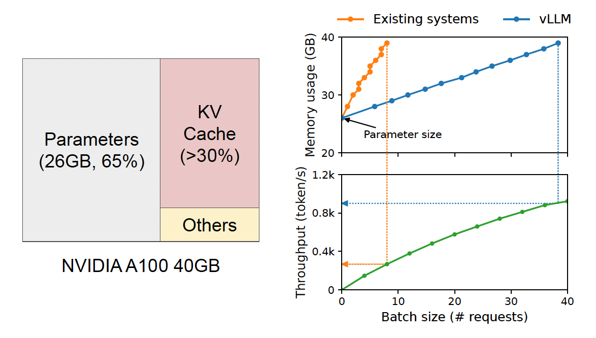
Optimizing only one of these is a job half-done. An efficient serving system must address both. The image below illustrates this breakdown, showing how the KV Cache can consume a substantial portion of GPU memory, often rivaling the model parameters themselves.
2. A New Frontier: Quantizing the KV Cache
Just as we can reduce the precision of model weights from FP16 to INT8 or INT4, we can apply the same principle to the tensors stored in the KV cache. This is known as KV cache quantization.
This is an incredibly powerful lever, especially for applications involving long contexts. As the sequence length increases, the size of the KV cache grows linearly and can easily surpass the memory required for the model weights. Halving the memory footprint of the KV cache can therefore free up enormous amounts of VRAM, allowing for longer contexts, larger batch sizes, or both.
To understand the mechanics and impact of this technique, please study the following material.
KV Cache Optimization: Memory Efficiency for Production LLMs ...
The article 'KV Cache Optimization' provides an excellent, concise explanation of KV cache quantization, including the different precision formats and how to enable them in a modern serving framework like vLLM.
Please read the section titled 'KV cache quantization'. Focus on understanding the concept, the different data types available (FP8, INT4), and the associated code example for enabling it in vLLM.
As the article details, modern GPUs like the NVIDIA Hopper and Blackwell series have native support for FP8 computation, making FP8 KV cache quantization nearly "free" in terms of performance, while halving the memory usage compared to FP16. This has become a standard optimization for production systems.
The following table starkly visualizes the benefits. Notice how the percentage of memory saved by KV Cache Quantization becomes more significant as the context window grows.

3. Measuring the Cumulative Impact: A Practical Exercise
Let's quantify the combined memory savings. We will perform a calculation-based exercise to estimate the total VRAM required to serve a Llama 3 8B model under different optimization scenarios. This is precisely the kind of back-of-the-envelope calculation an AI Systems Engineer performs to plan capacity.
Scenario:
- Model: Llama 3 8B (~8.03 billion parameters)
- Hardware: A single GPU with 24 GB of VRAM
- Workload: Batch size of 16, with a context length of 4096 tokens.
We will use the memory formulas you learned in Module 3. Recall that total memory is approximately:
(We'll ignore activation memory for this estimation, as it's typically smaller and more complex to model, but the weights and KV cache are the dominant factors).
Llama 3 8B Architecture Details:
num_layers= 32num_heads= 32head_dim= 128
Step 1: Baseline (FP16 Model, FP16 KV Cache)
- Model Weights Memory:
- KV Cache Memory:
- Total Estimated VRAM: 15.0 GB + 3.2 GB = 18.2 GB
Step 2: Model Quantization Only (INT4 AWQ Model, FP16 KV Cache)
- Model Weights Memory: We'll use a factor of ~0.55 bytes/param for a 4-bit quantized model to account for quantization scales and metadata.
- KV Cache Memory: Unchanged from baseline.
- Total Estimated VRAM: 4.1 GB + 3.2 GB = 7.3 GB
Step 3: KV Cache Quantization Only (FP16 Model, FP8 KV Cache)
- Model Weights Memory: Unchanged from baseline.
- KV Cache Memory: We now use 1 byte per element for FP8.
- Total Estimated VRAM: 15.0 GB + 1.6 GB = 16.6 GB
Step 4: Combined Optimization (INT4 AWQ Model, FP8 KV Cache)
- Model Weights Memory: Same as Step 2.
- KV Cache Memory: Same as Step 3.
- Total Estimated VRAM: 4.1 GB + 1.6 GB = 5.7 GB
Summary of Savings
| Optimization Scenario | Model VRAM | KV Cache VRAM | Total VRAM | % Savings (vs. Baseline) |
|---|---|---|---|---|
| 1. Baseline (FP16/FP16) | 15.0 GB | 3.2 GB | 18.2 GB | 0% |
| 2. Model Quant (INT4/FP16) | 4.1 GB | 3.2 GB | 7.3 GB | 60% |
| 3. KV Cache Quant (FP16/FP8) | 15.0 GB | 1.6 GB | 16.6 GB | 9% |
| 4. Combined (INT4/FP8) | 4.1 GB | 1.6 GB | 5.7 GB | 69% |
This analysis demonstrates the immense power of a combined optimization strategy. By quantizing both the model and the KV cache, we reduced the VRAM footprint from over 18 GB to under 6 GB—a nearly 70% reduction. On our 24 GB GPU, this frees up enough memory to potentially 3-4x the batch size, dramatically increasing server throughput.
4. Implementation in vLLM
Putting this into practice is surprisingly straightforward with modern serving frameworks. vLLM, for example, allows you to enable these optimizations with simple command-line arguments.
Systematic Framework for vLLM Inference Optimization
This article, 'Systematic Framework for vLLM Inference Optimization', provides a practical guide to applying various optimizations. We'll focus on the specific flags for quantization.
Review the section '1.2 Quantization Strategy'. Note the command-line arguments used to run vLLM with a quantized model, specifically --quantization awq.
To implement our fully optimized scenario (INT4 model, FP8 KV cache), you would combine the flags you've seen in today's resources:
```grasp
{
  "type": "exercise",
  "id": "9c19f77b-5177-4247-b04f-246c43596865"
}
Example vLLM command combining both optimizations
python -m vllm.entrypoints.openai.api_server
--model <path_to_your_awq_quantized_model>
--quantization awq
--kv-cache-dtype fp8
--gpu-memory-utilization 0.9
By launching the server with these flags and monitoring your GPU with `nvidia-smi`, you could empirically verify the memory savings we calculated.


### Conclusion

In this lesson, you have integrated two of the most important memory optimization paradigms in LLM serving. You've moved beyond treating model size and runtime state as separate problems and learned to attack them in a unified way.

**Key Takeaways:**

*   Total VRAM usage is a sum of its parts, primarily **model weights** and the **KV cache**.
*   **KV cache quantization** is a powerful technique that complements model quantization, with its benefits amplifying at longer context lengths.
*   By combining model quantization (e.g., INT4-AWQ) with KV cache quantization (e.g., FP8), you can achieve cumulative memory savings that are far greater than either technique in isolation.
*   This combined approach is the standard for maximizing the efficiency and throughput of a single GPU, allowing you to serve larger batches and longer sequences than would otherwise be possible.

**Preview of the Next Lesson:**

We have now reached the limits of what we can optimize on the model and memory management level for a single forward pass. However, our GPU is often still underutilized, waiting for work. The next major bottleneck is how we schedule and batch incoming requests. In the next module, you will move from these *static* optimizations to *dynamic runtime* optimizations by implementing a **continuous batching scheduler**, the core engine behind high-throughput LLM serving systems.