KV Cache for Autoregressive Decoding: Memory Analysis

Introduction

In our last lesson, we generalized our attention mechanism to Grouped-Query Attention (GQA), analyzing how it provides a crucial trade-off between the memory footprint of the KV cache and model quality. We focused on the static aspect of the cache—how its potential size is determined by the model's architecture (number of layers, heads, etc.).

Today, we shift from static analysis to dynamic, runtime behavior. Your learning outcome for this lesson is to implement a basic KV cache for autoregressive decoding and measure its memory growth over the generation sequence.

We will explore why simply re-running the model for each new token is computationally prohibitive and how the KV cache solves this problem. You will modify a transformer's forward pass and generation loop to implement this caching mechanism from scratch. This is a foundational skill in LLM systems engineering, as it's the core optimization that makes large-scale text generation feasible.

The Problem: Quadratic Complexity in Autoregressive Decoding

Autoregressive generation works by predicting one token at a time, appending it to the input sequence, and then feeding the entire new sequence back into the model to generate the next token. While simple, this approach is incredibly inefficient.

At each step, the self-attention mechanism must compute relationships between the new token and all previous tokens. This means that for a sequence of length $T$, the computations for keys and values for the first $T-1$ tokens are performed repeatedly. This redundant work causes the overall computation to scale quadratically with the sequence length, i.e., $O(T^2)$.

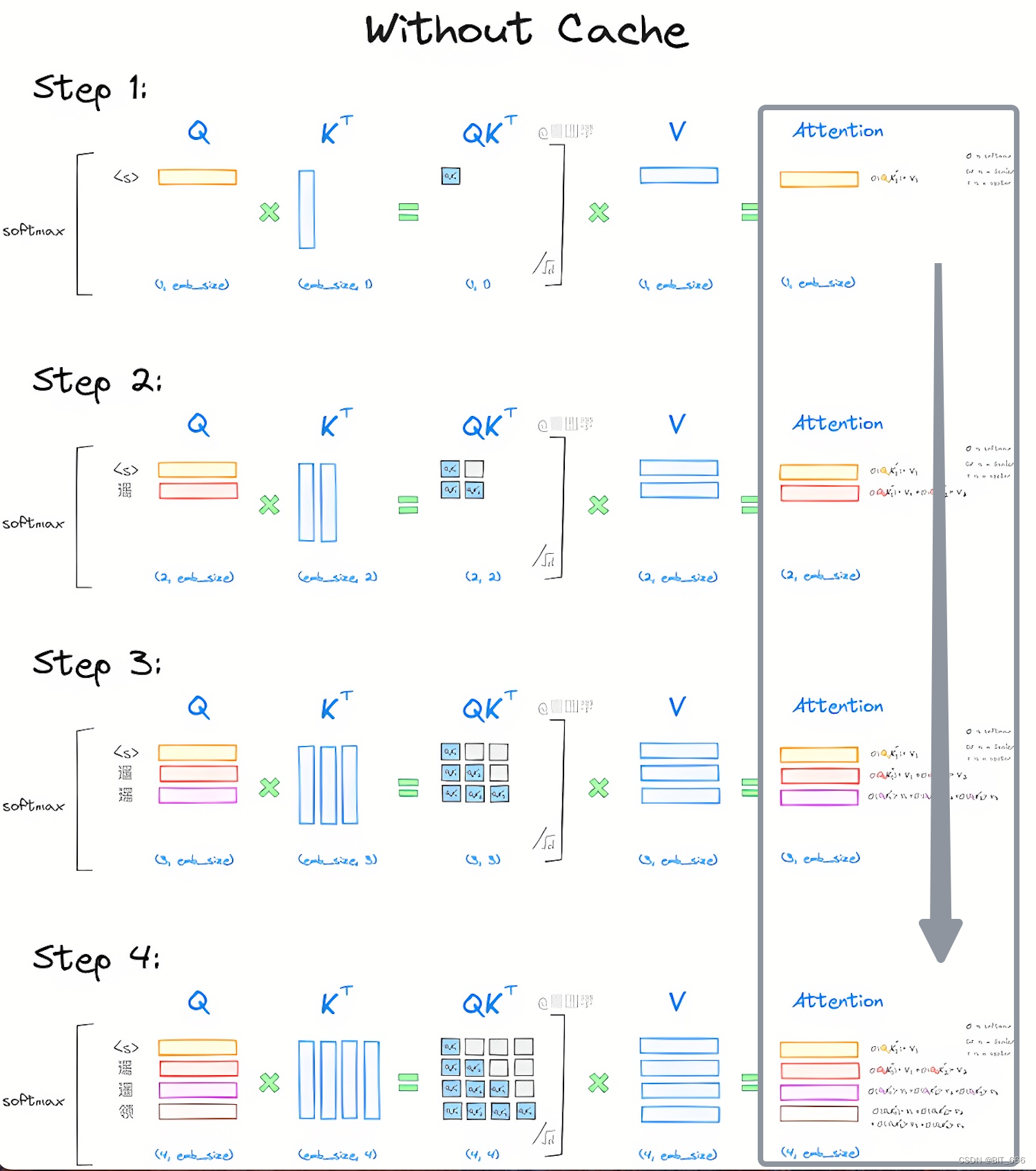
To get a clear, visual understanding of this "triangle of waste," let's watch a short video that breaks down the problem.

The video makes it clear: as the generated sequence gets longer, the model spends most of its time re-calculating things it already knew. For a systems engineer, this is a five-alarm fire of inefficiency that needs to be extinguished.

The Solution: Caching Keys and Values

The solution is conceptually simple: if we are recomputing the same key and value vectors, let's just save them. This is the essence of the Key-Value (KV) cache.

The new workflow becomes:

1. Prefill Phase: The model processes the initial prompt tokens all at once. It computes the key and value vectors for every token in the prompt and stores them in the cache.
2. Decode Phase (Token-by-Token): For each subsequent generation step, the model only takes the single newest token as input. It computes the K and V vectors for just this one token and appends them to the cache. The query vector for this new token can then attend to the full history of keys and values stored in the cache.

This transforms the computation from $O(T^2)$ to $O(T)$, as each step now involves a constant amount of new computation (for the new token) and an attention operation whose cost grows linearly with the cache size.

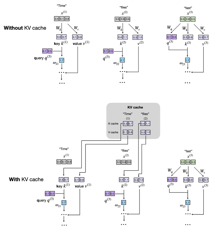
Let's continue with the video, which now explains this efficient workflow.

Now that the "why" and "what" are clear, we'll turn to the "how" by implementing this mechanism in PyTorch.

Hands-On: Implementing a Basic KV Cache

We will implement a KV cache by modifying a simple decoder-only transformer. We'll use Sebastian Raschka's excellent article as a guide, which provides a very clear, from-scratch implementation designed for readability.

Now, let's translate this into code. Create a Python script and build the following components. The implementation is based on the one in the article you just read.

1. The MultiHeadAttention Module

Modify your MultiHeadAttention class (or create a new one) to include the caching logic.

import torch
import torch.nn as nn
import time
import matplotlib.pyplot as plt




# A simplified MultiHeadAttention with KV caching
class CausalSelfAttention(nn.Module):
    def __init__(self, d_model, num_heads, head_dim):
        super().__init__()
        self.d_out = d_model
        self.num_heads = num_heads
        self.head_dim = head_dim
        
        self.W_query = nn.Linear(d_model, d_model)
        self.W_key = nn.Linear(d_model, d_model)
        self.W_value = nn.Linear(d_model, d_model)
        self.out_proj = nn.Linear(d_model, d_model)




        # Register cache as buffers. Buffers are part of the module's state
        # but are not considered model parameters (i.e., not trained).
        self.register_buffer('cache_k', None)
        self.register_buffer('cache_v', None)

    def forward(self, x, use_cache=False):
        b, num_tokens, d_in = x.shape

        keys_new = self.W_key(x)
        values_new = self.W_value(x)
        queries = self.W_query(x)

        if use_cache:
            if self.cache_k is None:



                # First pass (prefill)
                self.cache_k = keys_new
                self.cache_v = values_new
            else:



                # Subsequent passes (decode)
                self.cache_k = torch.cat([self.cache_k, keys_new], dim=1)
                self.cache_v = torch.cat([self.cache_v, values_new], dim=1)
            
            keys = self.cache_k
            values = self.cache_v
        else:
            keys = keys_new
            values = values_new
        



        # Reshape for multi-head attention
        keys = keys.view(b, keys.shape[1], self.num_heads, self.head_dim).transpose(1, 2)
        values = values.view(b, values.shape[1], self.num_heads, self.head_dim).transpose(1, 2)
        queries = queries.view(b, num_tokens, self.num_heads, self.head_dim).transpose(1, 2)
        



        # Attention calculation
        attn_scores = queries @ keys.transpose(2, 3)



        # Causal mask
        mask = torch.triu(torch.ones(num_tokens, keys.shape[2]), diagonal=1).bool()
        attn_scores = attn_scores.masked_fill(mask, -torch.inf)
        
        attn_weights = torch.softmax(attn_scores / self.head_dim**0.5, dim=-1)
        context_vec = (attn_weights @ values).transpose(1, 2).reshape(b, num_tokens, self.d_out)
        
        return self.out_proj(context_vec)

    def reset_cache(self):
        self.cache_k = None
        self.cache_v = None

2. The Generation Loop

Next, create a generate function that uses this caching logic. Notice the if/else block: when use_cache is True, we first do a prefill and then loop, feeding only the single next_token_id to the model.

# A minimal TransformerBlock and GPTModel for the sake of a runnable example
class TransformerBlock(nn.Module):
    def __init__(self, d_model, num_heads, head_dim):
        super().__init__()
        self.attn = CausalSelfAttention(d_model, num_heads, head_dim)



        # In a real model, there would be FFN, LayerNorm, etc.

    def forward(self, x, use_cache=False):
        return self.attn(x, use_cache=use_cache)

    def reset_cache(self):
        self.attn.reset_cache()
        
class GPTModel(nn.Module):
    def __init__(self, vocab_size, d_model, num_layers, num_heads, head_dim):
        super().__init__()
        self.tok_emb = nn.Embedding(vocab_size, d_model)
        self.pos_emb = nn.Embedding(2048, d_model) # Max context length
        self.trf_blocks = nn.ModuleList([
            TransformerBlock(d_model, num_heads, head_dim) for _ in range(num_layers)
        ])
        self.current_pos = 0

    def forward(self, idx, use_cache=False):
        batch_size, seq_len = idx.shape
        
        if use_cache:
            pos_ids = torch.arange(self.current_pos, self.current_pos + seq_len).unsqueeze(0)
            self.current_pos += seq_len
        else:
            pos_ids = torch.arange(seq_len).unsqueeze(0)
            
        x = self.tok_emb(idx) + self.pos_emb(pos_ids)
        for block in self.trf_blocks:
            x = block(x, use_cache=use_cache)



        # In a real model, a final linear layer would project to vocab size
        return x # Returning hidden states for simplicity

    def reset_kv_cache(self):
        for block in self.trf_blocks:
            block.reset_cache()
        self.current_pos = 0

def generate(model, prompt_tokens, max_new_tokens, use_cache=True):
    model.eval()
    
    if use_cache:



        # Reset cache and position before starting a new generation
        model.reset_kv_cache()
        



        # 1. Prefill Phase
        with torch.no_grad():
            _ = model(prompt_tokens, use_cache=True) # Populate the cache
        
        next_token_id = torch.tensor([[0]]) # Dummy next token
        



        # 2. Decode Phase
        for _ in range(max_new_tokens):
            with torch.no_grad():



                # Pass only the newest token
                _ = model(next_token_id, use_cache=True)
    else:



        # Full sequence generation at each step
        full_sequence = prompt_tokens
        for _ in range(max_new_tokens):
            with torch.no_grad():
                _ = model(full_sequence, use_cache=False)
            



            # Append a dummy token to simulate growth
            next_token_id = torch.tensor([[0]]) 
            full_sequence = torch.cat([full_sequence, next_token_id], dim=1)

This implementation, while simplified, contains all the core logic for a functional KV cache.

Exercise: Measuring Memory Growth

Now for the measurement part of our learning outcome. Let's write a function to run the generation process step-by-step and record the size of the KV cache at each step. The number of elements (numel()) in the cache tensors is a direct proxy for memory usage.

Add this function to your script and run it.

def measure_cache_growth(model, prompt_len, max_new_tokens):
    """
    Measures the KV cache size at each step of autoregressive generation.
    Returns lists of tokens processed and cache sizes.
    """
    model.eval()
    model.reset_kv_cache()
    



    # --- Data tracking ---
    token_counts = []
    cache_sizes = []
    



    # --- Prefill Phase ---
    prompt_tokens = torch.zeros((1, prompt_len), dtype=torch.long)
    with torch.no_grad():
        _ = model(prompt_tokens, use_cache=True)
    



    # Measure after prefill
    current_tokens = prompt_len
    total_elements = 0
    for block in model.trf_blocks:



        # Cache = K + V. Size is Batch * SeqLen * NumHeads * HeadDim
        # We simplify by just getting the number of elements.
        total_elements += block.attn.cache_k.numel()
        total_elements += block.attn.cache_v.numel()

    token_counts.append(current_tokens)
    cache_sizes.append(total_elements)




    # --- Decode Phase ---
    for i in range(max_new_tokens):
        next_token_id = torch.zeros((1, 1), dtype=torch.long)
        with torch.no_grad():
            _ = model(next_token_id, use_cache=True)
        
        current_tokens += 1
        total_elements = 0
        for block in model.trf_blocks:
            total_elements += block.attn.cache_k.numel()
            total_elements += block.attn.cache_v.numel()
            
        token_counts.append(current_tokens)
        cache_sizes.append(total_elements)
        
    return token_counts, cache_sizes




# --- Model Configuration ---
D_MODEL = 512
NUM_LAYERS = 6
NUM_HEADS = 8
HEAD_DIM = D_MODEL // NUM_HEADS
VOCAB_SIZE = 1000




# --- Experiment Parameters ---
PROMPT_LEN = 10
MAX_NEW_TOKENS = 100




# --- Run the measurement ---
model = GPTModel(VOCAB_SIZE, D_MODEL, NUM_LAYERS, NUM_HEADS, HEAD_DIM)
tokens, sizes = measure_cache_growth(model, PROMPT_LEN, MAX_NEW_TOKENS)




# --- Plotting the results ---
plt.figure(figsize=(10, 6))
plt.plot(tokens, sizes, marker='o', linestyle='-')
plt.title('KV Cache Size vs. Sequence Length')
plt.xlabel('Total Sequence Length (Tokens)')
plt.ylabel('KV Cache Size (Number of Elements)')
plt.grid(True)
plt.show()




# --- Theoretical Calculation ---
# Total elements = 2 (for K,V) * L * B * S * N_h * D_h
# Here B=1, S=current_tokens, N_h=NUM_HEADS, D_h=HEAD_DIM
final_tokens = tokens[-1]
theoretical_size = 2 * NUM_LAYERS * 1 * final_tokens * NUM_HEADS * HEAD_DIM
print(f"Measured size at {final_tokens} tokens: {sizes[-1]}")
print(f"Theoretical size at {final_tokens} tokens: {theoretical_size}")

When you run this code, you will see a plot showing a straight line. This confirms our understanding: the KV cache size grows linearly with the sequence length. The total memory required is given by the formula:

Where:

• $L$: number of layers
• $B$: batch size
• $S$: sequence length
• $N_{kv}$: number of key-value heads
• $D_h$: dimension of each head

Your measurement exercise empirically validates the linear relationship with $S$.

Conclusion

In this lesson, you have moved from theory to practice by implementing one of the most fundamental optimizations in LLM inference. You now have a robust mental and practical model for how the KV cache works.

Key Takeaways:

• Naive autoregressive decoding has a quadratic compute cost ($O(T^2)$) due to redundant calculations in the attention mechanism.
• The KV cache solves this by storing previously computed key and value tensors, reducing the complexity to linear ($O(T)$).
• Implementing a KV cache requires modifying the attention forward pass to append new K/V pairs and updating the generate loop to feed only the newest token after an initial prefill step.
• The memory footprint of the KV cache grows linearly with the sequence length, which can become a major bottleneck for long contexts.

Preview of the Next Lesson:

Our basic cache grows indefinitely until it exhausts GPU memory. This is not a viable strategy for production systems that need to handle long sequences or high concurrency. In our next lesson, we will address this limitation. You will implement and compare different KV cache eviction strategies (e.g., sliding window, token dropping) and evaluate their impact on generation quality. This will introduce you to the trade-offs required when memory is a finite and precious resource.