Configuring Inverter Power and Reactive Limits from Ratings and Capability Curves

Welcome. This module shifts from network topology into the steady-state representation of a utility-scale renewable plant. Before transformer, collector, and POI-control details can be trusted, the inverter-equivalent machine must have credible ratings and limits. A power-flow case can converge with almost any numbers entered into the Machine Data Record; the engineering task is making those numbers correspond to the facility that will actually be built and studied.

By the end of this lesson, you will be able to take inverter schedules and capability-curve data and populate the PSS®E fields for MBASE, PGEN, PMAX, PMIN, QMAX, and QMIN without confusing inverter-terminal capability, station service, interconnection losses, and POI injection.

---

1. Start with the correct electrical boundary

The central modeling distinction is between what an inverter can do at its AC terminals and what the project delivers or absorbs at the point of interconnection (POI).

A project’s active-power quantities commonly fall into three layers:

Layer	Meaning	Typical use in the PSS®E project model
Gross inverter-terminal output	AC real power produced by the inverter or aggregate inverter block	Establishes inverter $P_{\max }$ and the operating-point $P_{\text{gen}}$ before internal loads/losses
Output after station service	Gross output less auxiliary demand connected at the inverter or collector level	Requires an explicitly modeled station-service load if it is electrically inside the project boundary
Net POI injection	Output reaching the transmission system after station service and interconnection-facility losses	Must match the studied export limit, ERIS quantity, or scenario definition at the POI

For an exporting solar facility,

$$P_{\text{POI}}=P_{\text{inverter gross}}-P_{\text{station service}}-P_{\text{facility losses}}$$

For example, suppose a plant has 120 MW of aggregate inverter AC output, 2 MW of modeled station service, and 3 MW of collector, transformer, and gen-tie losses at the selected dispatch. Its net POI injection is approximately:

$$120-2-3=115\text{MW}$$

The inverter-equivalent machine can legitimately have $P_{\max }=120$ MW, while the POI export is 115 MW. Setting $P_{\max }$ to 115 MW simply because that is the requested POI capability would erase the physical distinction between capability and losses.

For a BESS in charging operation, the sign reverses at the machine: negative $P_{\text{gen}}$ means the machine is absorbing real power from the grid. If 97 MW is absorbed at the aggregate inverter terminals and there are 3 MW of electrical losses between that terminal and the POI, the POI sees approximately 100 MW of withdrawal. Thus, a declared 100 MW charging demand at the POI does not necessarily mean $P_{\min }=-100$ MW at the inverter-terminal machine.

The precise project boundary and required convention come from the applicable ISO/RTO, transmission owner, and interconnection agreement. The ISO-NE guidance below is useful because it makes the terminal-to-POI distinction explicit. It is an example of sound modeling discipline, not a substitute for ERCOT, SPP, WECC, or utility-specific requirements.

---

2. What each PSS®E machine field means

In the PSS®E steady-state Machine Data Record, the relevant values are expressed in MW, Mvar, and MVA, not per unit.

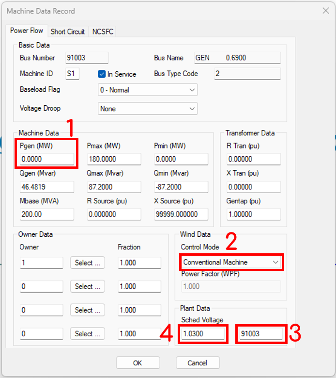
Assume the electrical topology, generator bus, and transformer representation have already been created. The fields then have distinct purposes:

Field	Meaning	How to establish it
PGEN	Initial scheduled real-power output for the particular solved case	Set from the study scenario; it is not necessarily the maximum capability
PMAX	Maximum real-power generation at the machine’s modeled boundary	Use maximum intended gross AC output of the inverter aggregate
PMIN	Minimum real-power output at that boundary	Usually zero for solar; often negative for a BESS to represent charging
QGEN	Initial reactive schedule or initial solution value	Use a plausible initial value; under voltage control PSS®E will solve reactive output subject to limits
QMAX	Largest permitted positive reactive injection	Use the documented lagging, vars-supplying limit at the relevant active-power point
QMIN	Largest permitted reactive absorption, entered as a negative number	Use the documented leading, vars-absorbing limit with the correct PSS®E sign
MBASE	MVA base/rating for this machine equivalent	Use the aggregate AC inverter nameplate MVA represented by that machine

Two conventions deserve particular attention:

1. Positive $P_{\text{gen}}$ represents real-power generation into the network. A discharging BESS has positive $P_{\text{gen}}$; a charging BESS has negative $P_{\text{gen}}$.

2. In the conventional generator sign convention, positive $Q_{\text{gen}}$ is reactive injection into the network. Therefore, a generator that can provide $+40$ Mvar and absorb $40$ Mvar would normally have:

$$Q_{\max }=+40\text{Mvar}$$ $$Q_{\min }=-40\text{Mvar}$$

Do not transfer signs from an OEM curve without first checking its stated convention. Some documents use “leading” and “lagging” from the facility, grid, or load viewpoint; the labels may be correct while the implied algebraic sign differs from the PSS®E entry convention.

---

3. MBASE is an AC MVA rating, not the project’s MW export limit

For inverter-based resources, MBASE should represent the AC MVA nameplate of the inverter group represented by the machine record. It is not the DC PV array rating, the battery energy capacity in MWh, or automatically the POI MW limit.

If 60 identical inverters are each rated 2.2 MVA, then the aggregated equivalent is:

$$MBASE=60\times 2.2=132\text{MVA}$$

If those inverters each have a maximum AC real-power output of 2.0 MW, then:

$$P_{\max }=60\times 2.0=120\text{MW}$$

The fact that $P_{\max }$ is lower than MBASE is normal. It reflects an inverter design with MVA headroom, which may support reactive capability while delivering rated MW.

MBASE matters beyond the label in the dialog. It establishes the machine base used when interpreting certain impedance and dynamic-model quantities. An incorrect MBASE can therefore create an inconsistency that is initially hidden in the power flow but becomes consequential when the PSS®E dynamic model is introduced.

For a hybrid project, generally use separate equivalent machines for separate resource types, such as one solar equivalent and one BESS equivalent, unless the required modeling approach explicitly calls for a combined representation. Solar and storage have different $P_{\min }$ behavior, operating constraints, control chains, and often different capability curves. Combining them prematurely makes charging, discharging, curtailment, and reactive-capability assumptions difficult to audit.

The NYISO guideline provides a compact example of a regional submission convention: use an aggregate model where appropriate, set MBASE to total nameplate MVA, and set real and reactive limits from intended operation. Its specific ERIS and power-factor requirements are NYISO-specific, but its treatment of machine fields is broadly useful.

---

4. Convert a capability curve into credible Q limits

A capability curve defines which combinations of real and reactive power are feasible. It is more informative than a single power-factor number because reactive capability usually changes with real-power output, terminal voltage, temperature, current limit, and control mode.

At minimum, request or extract these points for each inverter type:

• AC MVA rating;
• maximum and minimum real power;
• lagging and leading reactive limits at rated real power;
• lagging and leading reactive limits at zero real power;
• any stated voltage range, thermal derating, or active/reactive-priority condition;
• whether values apply at inverter terminals, a collector bus, the GSU high side, or the POI.

A useful plausibility check comes from the apparent-power relation:

$$S^2=P^2+Q^2$$

If an inverter is rated $132$ MVA and produces 120 MW, its theoretical circular apparent-power limit would permit approximately:

$$\left|Q\right|=\sqrt{132^2-120^2}=54.2\text{Mvar}$$

But this is only an upper physical check, not a substitute for the manufacturer curve. The inverter may be contractually or technologically limited to 0.95 power factor at maximum MW. At 120 MW and 0.95 power factor, the corresponding reactive magnitude is:

$$\left|Q\right|=120\tan ({\cos }^{-1}(0.95))=39.4\text{Mvar}$$

Suppose the OEM capability table says the aggregate inverter block can:

• export up to 120 MW;
• supply or absorb 39.4 Mvar at 120 MW;
• supply or absorb 55 Mvar at zero MW;
• operate on a 132 MVA aggregate nameplate rating.

For a full-output solar power-flow case, a defensible initial machine entry is:

Parameter	Entry
MBASE	132 MVA
PMAX	120 MW
PMIN	0 MW
PGEN	120 MW before explicitly modeled station-service load and network losses
QMAX	+39.4 Mvar
QMIN	−39.4 Mvar

The values at zero MW remain essential evidence even though they are not directly represented by the same constant $Q_{\max }$ and $Q_{\min }$ entries in this full-output case.

The limitation of fixed QMAX and QMIN

The basic machine fields displayed in PSS®E are a pair of fixed reactive bounds. A real $P$-$Q$ curve is often non-rectangular: the available reactive range may be much larger at low real power than at rated output. Consequently, one pair of constant Q limits cannot automatically reproduce the entire capability curve at every dispatch.

Use this reasoning:

• For a single fixed-dispatch study, set $Q_{\max }$ and $Q_{\min }$ to the documented capability at that dispatch, accounting for the modeled electrical boundary.
• For multiple dispatch cases, update the limits for each operating point or use the documented/project-approved capability-curve treatment.
• Never use the maximum zero-MW reactive capability as a constant limit in a 100% output case unless the actual curve confirms it is available there.
• Never invent a larger capability merely to achieve a POI power-factor target. If the inverter limit is insufficient after collector and transformer reactive losses, model the actual switched shunts, STATCOM, SVC, or other installed reactive equipment separately.

This distinction prevents a common but consequential error: giving an inverter 55 Mvar of capability at 120 MW merely because it can provide 55 Mvar at zero MW.

---

5. A practical PSS®E entry workflow

Use a repeatable data trail rather than entering values from memory.

Step 1: Build a source-data sheet

For every machine equivalent, record:

• resource type and aggregate quantity;
• inverter manufacturer and model;
• number of units represented;
• individual and aggregate MW and MVA ratings;
• capability-curve revision and units;
• active-power limits;
• reactive limits at the selected active-power point;
• station-service location and MW;
• assumed dispatch and expected POI MW;
• source document, page, and revision.

This is the first part of a defensible study record. It also makes later comparison with PSCAD much easier.

Step 2: Decide the aggregation and boundary

Represent the same physical grouping used by the approved power-flow and dynamic-model package. If the power-flow model uses one aggregate solar inverter machine, its MBASE and limits must be the sums of the represented inverters. If solar and BESS are separate resources, preserve separate machine records unless instructed otherwise.

At this stage, distinguish the inverter terminal from the POI. Do not compensate for unknown losses by reducing MBASE. MBASE remains equipment MVA; losses belong in the modeled project network.

Step 3: Populate active-power fields

Enter:

• $P_{\max }$ from maximum intended gross AC generation;
• $P_{\min }$ from the minimum intended output, including a negative charging limit for storage where applicable;
• $P_{\text{gen}}$ from the particular scenario being solved.

For an interconnection-request base case, the project may be required to initialize at zero and be dispatched by the study organization. For an internal sensitivity case, initialize at the explicitly documented dispatch. These are different case conventions, so do not treat one as universally correct.

Step 4: Populate MBASE and reactive bounds

Enter aggregate inverter MVA in MBASE. Then enter QMAX and QMIN for the selected operating point using the OEM or approved capability curve, with PSS®E signs.

If the unit is intended to regulate voltage, the solved $Q_{\text{gen}}$ may move after the power flow is solved. It must remain between QMIN and QMAX. When a limit is reached, PSS®E can no longer maintain its voltage target solely through that machine; the resulting voltage and reactive flows are part of the study result, not a reason to silently expand the limits.

Step 5: solve, inspect, and document

After solving the power flow, check:

1. machine real output against the scenario;
2. machine reactive output against QMIN and QMAX;
3. station-service load and collector/transformer losses;
4. net MW and Mvar at the POI;
5. whether any machine is at a reactive limit;
6. whether the modeled POI capability remains consistent with the project data package.

The following short video segment is useful for locating the machine fields in PSS®E and seeing the order in which they are entered. Its numerical rules of thumb, such as setting $P_{\max }$ to a percentage above $P_{\text{gen}}$, are illustrative workflow choices—not substitutes for OEM ratings and approved project data.

---

6. BESS-specific preview: symmetric ratings are not guaranteed

A BESS machine is not simply a solar machine with a negative PGEN value. Before setting BESS limits, verify:

• whether maximum charge MW equals maximum discharge MW;
• whether the inverter MVA rating is the same in both directions;
• whether reactive capability changes in charge versus discharge;
• whether the battery PCS has state-of-charge, thermal, or auxiliary-load restrictions;
• whether the stated charging quantity is at the inverter terminals or the POI.

For a symmetric 100 MW / 110 MVA BESS equivalent, an initial representation might be:

$$P_{\max }=+100\text{MW}$$ $$P_{\min }=-100\text{MW}$$ $$MBASE=110\text{MVA}$$

However, those values are valid only if the equipment documentation supports symmetric operation at the chosen boundary. Charging losses, auxiliary consumption, and internal transformer losses must still be represented so that the net POI withdrawal is correct.

---

Key takeaways

• MBASE is the aggregate AC inverter MVA rating represented by the machine, not the PV DC rating, BESS MWh capacity, or POI export limit.
• PGEN is the case operating point; PMAX and PMIN are capability limits at the modeled machine boundary.
• Model station service and electrical losses explicitly so that inverter-terminal output and net POI injection are not confused.
• In normal PSS®E generator convention, reactive injection is positive: $Q_{\max }$ is the vars-supplying limit and $Q_{\min }$ is the negative vars-absorbing limit.
• Derive Q limits from the documented capability curve at the active-power operating point. Do not infer full-output capability from zero-output Mvar capability or from a generic power-factor assumption.
• A fixed pair of Q limits is not a complete $P$-$Q$ curve; document how limits are adjusted across study dispatches.

Next, the course applies these conventions specifically to standalone BESS charging and discharging dispatch, including signs, POI withdrawal/export, efficiency assumptions, and operating limits.