Defining Position–Velocity States in an Inertial Frame

Hello again. In the previous lesson, you defined a deliberately narrow Earth–satellite modelling brief: Newtonian gravity, point masses, a finite time horizon, and an explicit distinction between physical model, numerical method, and validation.

This lesson turns the phrase “simulate an orbit” into a precise data description. Before deriving gravity or selecting an integrator, we must decide from where motion is measured and exactly which numbers at an initial time determine the future model trajectory. By the end, you will be able to specify a suitable inertial frame and encode the position–velocity state for either one satellite or a general system of point masses.

---

A reference frame is part of the model

A coordinate system supplies axes and an origin. A reference frame adds a rule for how those axes and origin move through time. The distinction matters because Newton’s laws take their simplest form only in an inertial frame.

Operationally, a frame is inertial if an isolated object with zero net force travels at constant velocity:

$$\mathbf{a}=0⟹\mathbf{v}=\text{constant}.$$

Equivalently, it is a frame in which Newton’s second law has its usual form,

$$\mathbf{F}=m\mathbf{a},$$

with no extra, frame-induced forces.

A frame whose origin moves at constant velocity relative to an inertial frame, and whose axes remain parallel to the original axes, is also inertial. Let ${\mathbf{a}}_0$ be a fixed displacement and $\mathbf{U}$ a constant relative velocity between frames. Then the coordinates of the same particle transform as

$${\mathbf{r}}^{\prime }=\mathbf{r}-{\mathbf{a}}_0-\mathbf{U}t,$$

and therefore

$${\mathbf{v}}^{\prime }=\mathbf{v}-\mathbf{U},{\mathbf{a}}^{\prime }=\mathbf{a}.$$

Position and velocity depend on the observer. Acceleration does not change under this constant-velocity change of frame. That is why the dynamical law retains the same form.

A frame fixed to Earth’s surface does not meet this criterion. Earth rotates, so its surface-fixed axes continually change direction. A satellite that appears stationary in such a frame is nevertheless moving in a circle through inertial space and therefore has an acceleration. To use Newton’s laws in a rotating frame, we would need extra centrifugal and Coriolis terms. Those are real bookkeeping terms caused by the coordinate choice, not new physical interactions.

For the elementary orbital model, the economical decision is therefore:

Use non-rotating Cartesian axes, rather than axes attached to Earth’s surface.

We will return to rotating frames only in the optional three-body extension, where their benefits justify their extra terms.

---

The practical frame for the first Earth–satellite model

There are two related frame choices worth distinguishing.

An exact inertial choice for an isolated system

For a genuinely isolated collection of point masses, a barycentric inertial frame is the cleanest choice. Its origin is the system’s centre of mass and its axes do not rotate. Once chosen, the centre of mass is at rest or moves with constant velocity, so this is an inertial frame.

This will be the natural frame for the later full two-body and $N$-body simulations, where every body responds to every other body’s gravity.

A useful approximation for the initial satellite model

For the first restricted Earth–satellite model, we use an Earth-centred inertial-like frame, conventionally called an Earth-Centred Inertial or ECI frame:

• origin: Earth’s centre of mass;
• $z$-axis: approximately along Earth’s rotation axis toward the North Pole;
• $x$- and $y$-axes: lie in Earth’s equatorial plane;
• orientation: the axes do not rotate once per day with Earth’s surface;
• handedness: choose a right-handed system, so that $x$, $y$, and $z$ obey the usual right-hand convention.

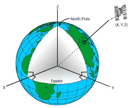
The diagram captures the geometric core of ECI: Earth may rotate beneath the axes, but the axes themselves do not turn with the planet.

Strictly speaking, an Earth-centred frame is not perfectly inertial in the real Solar System: Earth accelerates around the Sun and experiences smaller perturbations from the Moon and planets. In our initial model, those external effects are deliberately omitted. In addition, the satellite’s effect on Earth is neglected under the test-particle approximation. Within that stated idealisation, treating the Earth-centred origin as fixed is consistent and highly useful.

This gives a good rule for your model brief:

Model	Appropriate default coordinates
Satellite treated as a test particle around fixed Earth	Earth-centred, non-rotating Cartesian coordinates
Earth and Moon both move under mutual gravity	Barycentric inertial Cartesian coordinates
General isolated $N$-body system	Barycentric inertial Cartesian coordinates
Ground track or motion as seen by an observer on Earth	Earth-fixed rotating coordinates, with appropriate transformation or fictitious terms

Do not use “Earth-centred” as a synonym for “Earth-fixed.” An Earth-centred frame may have a rotating origin-independent set of axes, as in an Earth-fixed terrestrial frame, or non-rotating axes, as in ECI. The axis behaviour is the decisive difference.

For a reproducible real-data simulation, the frame specification must eventually be more explicit: for example, an ECI convention tied to a stated epoch such as J2000. For now, state the essential convention plainly:

Positions and velocities are Earth-centred Cartesian vectors in a right-handed, non-rotating frame.

---

From physical objects to a dynamical state

Suppose body $i$ has constant mass $m_i$. In a chosen inertial Cartesian frame, define its position and velocity by

$${\mathbf{r}}_i(t)=\left[\begin{array}{c}{x}_i(t)\\ y_i(t)\\ z_i(t)\end{array}\right],{\mathbf{v}}_i(t)={\dot{\mathbf{r}}}_i(t)=\left[\begin{array}{c}{v}_{x,i}(t)\\ v_{y,i}(t)\\ v_{z,i}(t)\end{array}\right].$$

Both are three-dimensional vectors. The position says where the point mass is; the velocity says how that position is changing at that instant.

For the restricted Earth–satellite problem, Earth is fixed at the origin by model assumption. The satellite’s state is thus the six-dimensional object

$$\mathbf{y}(t)=\left[\begin{array}{c}\mathbf{r}(t)\\ \mathbf{v}(t)\end{array}\right]=\left[\begin{array}{c}x(t)\\ y(t)\\ z(t)\\ v_x(t)\\ v_y(t)\\ v_z(t)\end{array}\right].$$

At a selected initial epoch $t_0$, the initial state is

$${\mathbf{y}}_0=\mathbf{y}(t_0)=\left[\begin{array}{c}{\mathbf{r}}_0\\ {\mathbf{v}}_0\end{array}\right].$$

It is important that position alone is not a state sufficient for orbital prediction. Two satellites can pass through exactly the same position with different velocities: one might be moving tangentially in a near-circular orbit, another could be plunging radially toward Earth, and a third could be escaping. Their future motions are different. The pair $(\mathbf{r},\mathbf{v})$, together with model parameters and the chosen frame, resolves that ambiguity.

This is the first appearance of a central applied-mathematics idea: the state is the smallest collection of quantities that, at the present time, contains all information the model needs to determine its future evolution.

At this point, the gravitational law has not yet been derived. But you already know its eventual structural role:

$$\dot{\mathbf{r}}=\mathbf{v},$$

while the velocity derivative will be specified by gravitational acceleration in the next lesson.

---

The state of $N$ point masses

For $N$ point masses, assemble every position and velocity at the same time $t$:

$$\mathbf{y}(t)=\left[\begin{array}{c}{\mathbf{r}}_1(t)\\ ⋮\\ {\mathbf{r}}_N(t)\\ {\mathbf{v}}_1(t)\\ ⋮\\ {\mathbf{v}}_N(t)\end{array}\right]\in {\mathbb{R}}^{6N}.$$

The system has $6N$ dynamical coordinates:

• $3N$ position coordinates;
• $3N$ velocity coordinates.

The masses

$$m_1,\dots ,m_N$$

are generally parameters, not components of the state, because the basic Newtonian model assumes they are constant. If we later model a rocket burning fuel, its mass would become time-dependent and would need separate treatment. That is outside the boundary of the present model.

For two bodies, a transparent flattened ordering is

$$\mathbf{y}={\left[\begin{array}{cccccccccccc}{x}_1& y_1& z_1& x_2& y_2& z_2& v_{x,1}& v_{y,1}& v_{z,1}& v_{x,2}& v_{y,2}& v_{z,2}\end{array}\right]}^{\mathsf{T}}.$$

The ordering is conventional, not mathematical. You could interleave each body’s position and velocity instead. What matters is that one ordering is selected, documented, and used consistently by:

1. the initial-condition constructor;
2. the force or acceleration function;
3. the numerical integrator;
4. the diagnostic and plotting code.

For the present course, we will use a more scalable internal representation before flattening for an ODE solver:

# All positions and velocities use one chosen frame and one chosen unit system.
positions = np.array([
    [x1, y1, z1],
    [x2, y2, z2],
], dtype=float)                 # shape: (N, 3)

velocities = np.array([
    [vx1, vy1, vz1],
    [vx2, vy2, vz2],
], dtype=float)                 # shape: (N, 3)

state = np.concatenate((
    positions.ravel(),
    velocities.ravel(),
))                              # shape: (6 * N,)

This format has two advantages:

• positions[i] and velocities[i] visibly refer to body $i$;
• the flat state vector has exactly the form expected by many numerical ODE interfaces.

For a single test-particle satellite, positions and velocities each have shape $(1,3)$, while the flattened state has six entries. For a later Sun–Earth–Moon model, their shapes would be $(3,3)$, and the flattened state would have eighteen entries.

---

Coordinate values are incomplete without metadata

An array such as

[7000.0, 0.0, 0.0, 0.0, 7.5, 0.0]

is not yet a scientifically interpretable state. It becomes one only when accompanied by its conventions. It might mean a satellite at $7000$ km from Earth’s centre, travelling at $7.5$ km/s in the positive $y$ direction. Or it could represent entirely different physical scales if the units are metres and metres per second.

Every saved initial condition should therefore carry at least the following metadata:

Item	Example for the first model	Why it matters
Epoch	$t_0=0$ s, or a documented calendar time	States at different times cannot be combined casually.
Frame	Earth-centred, non-rotating Cartesian	Defines the meaning of every component.
Origin	Earth’s centre of mass	States what $\mathbf{r}=0$ means.
Axis convention	Right-handed; $z$ northward	Prevents silent sign or orientation errors.
Distance unit	km	Must agree with gravitational parameters and plotting.
Time unit	s	Determines the unit of velocity and acceleration.
Body ordering	Earth first, satellite second, for example	Prevents applying forces to the wrong body.
Mass ordering	Matches body ordering	Required once mutual gravity is included.

For the early satellite-only model, a readable specification might be:

$${\mathbf{r}}_0=\left[\begin{array}{c}7000\\ 0\\ 0\end{array}\right]\text{ km},{\mathbf{v}}_0=\left[\begin{array}{c}0\\ 7.5\\ 0\end{array}\right]{\text{ km s}}^{-1}.$$

This places the satellite in the equatorial plane, initially on the positive $x$-axis, moving initially in the positive $y$-direction. The numbers are illustrative rather than yet a claimed circular-orbit prescription; later lessons will derive exactly how velocity must be chosen for a specified Keplerian orbit.

The frame and units also make a quick dimensional check possible. If position is in km and time is in s, then velocity must be in km/s. A position in metres paired accidentally with a gravitational parameter in ${\text{km}}^3{\text{/s}}^2$ can generate a visually dramatic but physically meaningless trajectory.

---

Relative states versus absolute states

There is one last distinction that will prevent confusion later.

In an inertial frame, let the absolute positions of two bodies be ${\mathbf{R}}_1$ and ${\mathbf{R}}_2$. Their relative position and relative velocity are

$$\mathbf{r}={\mathbf{R}}_2-{\mathbf{R}}_1,\mathbf{v}={\dot{\mathbf{R}}}_2-{\dot{\mathbf{R}}}_1.$$

For the current restricted Earth–satellite model, $\mathbf{r}$ is simply “the satellite’s Earth-centred position,” because Earth has been fixed at the origin by assumption.

For the full two-body problem, however, both Earth and satellite move in an inertial barycentric frame. Then the complete inertial state has twelve coordinates, but the relative state has six. In the next module, you will derive why the coupled twelve-coordinate system can be reduced in a principled way to relative motion plus centre-of-mass motion. For now, do not assume that “putting one massive body at the origin” is automatically an inertial transformation: it is justified here by the test-particle approximation, not by a general coordinate trick.

A useful implementation habit is to make the distinction visible in variable names:

R_earth, R_satellite       # absolute positions in a barycentric frame
V_earth, V_satellite       # absolute velocities

r_satellite_earth = R_satellite - R_earth
v_satellite_earth = V_satellite - V_earth

That naming discipline becomes especially valuable when the simulator grows from one moving satellite to a genuinely interacting $N$-body system.

---

A state-definition checklist

Before any integration begins, write a short state header in the notebook, configuration file, or model brief:

• Bodies: Which point masses are included, and in what order?
• Model parameters: Which masses and gravitational constants are fixed?
• Frame: Is it barycentric inertial or Earth-centred non-rotating?
• Axes: What do positive $x$, $y$, and $z$ mean?
• Units: Are position, velocity, mass, and time mutually consistent?
• Epoch: At what common time are the values specified?
• State layout: Are all positions followed by all velocities, or is another convention used?
• Approximation: Is a central body fixed, or are all bodies dynamically evolved?

This is not administrative overhead. It is the minimum information needed for someone else, or your future self, to reproduce the physical meaning of the simulation.

---

Key takeaways

An inertial frame is one in which force-free bodies move at constant velocity and Newton’s laws need no fictitious forces. A non-rotating Earth-centred frame is an appropriate approximation for the initial restricted Earth–satellite model; a barycentric inertial frame is the principled default once multiple bodies move mutually.

For each point mass, the dynamical state consists of position and velocity:

$$({\mathbf{r}}_i,{\mathbf{v}}_i).$$

For $N$ point masses, the full state has $6N$ scalar components. Masses are fixed model parameters in the basic Newtonian formulation, and every state vector must be accompanied by frame, unit, epoch, and ordering conventions.

Next, we will derive the vector gravitational acceleration of one point mass acting on another, including why the compact factor $\Vert \mathbf{r}{\Vert }^{-3}\mathbf{r}$ encodes both inverse-square magnitude and inward direction.