Algorithmic Invariant Tracing

In our last lesson, we focused on building a set of high-quality test cases. This methodical process helps confirm our understanding of a problem and provides a safety net for developing a solution. Now, we'll put those test cases to work by learning how to manually execute an algorithm on paper, a technique called tracing.

This lesson will show you how to use a trace table to simulate an algorithm's execution step-by-step. This powerful tool demystifies what code actually does, transforming an abstract set of instructions into a concrete, observable process. As we trace, we will also learn to identify a special kind of property called a loop invariant—a condition that remains true throughout the execution of a loop. Recognizing these invariants is a key step in moving from "I think this works" to "I can explain why this works," building your confidence and analytical skills.

What is Tracing?

Tracing, or "dry running," is the process of simulating a program's execution by hand. You act as the computer, tracking the value of each variable as the algorithm progresses line by line. This is an indispensable skill for both debugging your own code and understanding an unfamiliar algorithm.

The most common tool for this is a trace table. It's a simple table where columns represent variables, conditions, or outputs, and rows represent a step in the algorithm's execution.

The following short video provides a great introduction to the concept of dry running with trace tables.

As you saw, a trace table makes the flow of data visible. Let's look at another static example to solidify this.

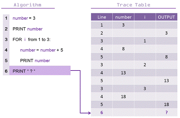
A Guided Tracing Example

Let's work through a complete example together. We will use the Linear Search algorithm, a fundamental search technique. The goal of linear search is to find the first occurrence of a specific item in a list by checking each element one by one.

The following document provides a detailed, step-by-step guide to tracing this algorithm. We will focus on the process itself, not just the final result.

From Tracing to Proving: Loop Invariants

Tracing shows you what an algorithm does on a specific input. But to gain true confidence, you need to understand why it works for all valid inputs. This is where the concept of a loop invariant comes in.

A loop invariant is a property or condition that is true before a loop starts, remains true after every single iteration of the loop, and gives you a useful guarantee when the loop finishes.

This idea is explained beautifully in the following article, which frames it as a practical tool for interview settings, aligning perfectly with your goals.

Let's apply this thinking to the linear search algorithm we just traced. A powerful invariant for the linear search loop is:

At the start of each iteration i, the itemToFind is not present in the subarray arrayToSearch[0...i-1] that has already been checked.

Let's verify this invariant:

• Initialization (Before the loop): The loop starts with i = 0. The subarray arrayToSearch[0...-1] is empty. The statement "the item is not in the empty subarray" is true. The invariant holds.
• Maintenance (During each iteration): Assume the invariant is true at the start of an iteration i. We then check arrayToSearch[i]. If it's not the item, we move to iteration i+1. Now, at the start of the new iteration, we have checked the subarray arrayToSearch[0...i], and the item was not in it. So the invariant holds for the next step.
• Termination (After the loop): The loop ends for one of two reasons:
  1. The item is found at index i. The algorithm correctly stops and reports the index.
  2. The loop finishes because i has gone through the entire array. The invariant tells us that the itemToFind was not in arrayToSearch[0...n-1] (where n is the array length). This proves that the item is not in the array at all, which is the correct conclusion.

This way of thinking—establishing a property and ensuring your code maintains it—is a cornerstone of algorithmic reasoning. It helps you build correct solutions from the ground up, rather than just hoping they work.

For a slightly more formal but still accessible explanation, the following video from a Carnegie Mellon course introduces loop invariants clearly.

Your Turn: An Exercise

Now it's your turn to practice. Consider the following simple algorithm written in pseudocode, which is designed to calculate the factorial of a non-negative integer n. (e.g., factorial of 4 is 4 * 3 * 2 * 1 = 24).

Algorithm: CalculateFactorial(n)

1. result = 1
2. i = 1
3. WHILE i <= n:
4. result = result * i
5. i = i + 1
6. END WHILE
7. RETURN result

Your Tasks:

1. Trace: Create a trace table for CalculateFactorial(4). Your table should have columns for the line number, n, i, result, and the condition i <= n.
2. Identify Invariant: State a loop invariant that relates result and i. What property is true at the start of every iteration of the WHILE loop?

Click here to see the solution.

1. Trace Table for CalculateFactorial(4)

Line	n	i	result	i <= n
1	4		1
2	4	1	1
3	4	1	1	True
4	4	1	1
5	4	2	1
3	4	2	1	True
4	4	2	2
5	4	3	2
3	4	3	2	True
4	4	3	6
5	4	4	6
3	4	4	6	True
4	4	4	24
5	4	5	24
3	4	5	24	False
7	4	5	24

(Note: Your trace table might have a slightly different format, for example, only showing a new row when a variable changes. The key is that the sequence of values is the same.)

2. Loop Invariant

A suitable loop invariant is:

At the beginning of each loop iteration, result holds the value of (i-1)! (factorial of i-1).

Let's check it:

• Initialization: Before the first iteration, i = 1. The invariant claims result should be (1-1)! = 0!. By definition, 0! = 1. The code initializes result = 1, so the invariant holds.
• Maintenance: Assume at the start of an iteration, result = (i-1)!. The loop body calculates new_result = result * i, which is (i-1)! * i, which equals i!. Then it increments i to i+1. So at the start of the next iteration, the new i is i+1 and the result is i!, which is (new_i - 1)!. The invariant is maintained.
• Termination: The loop terminates when i = n+1. The invariant tells us that result now holds the value of (i-1)!, which is ((n+1)-1)! = n!. The algorithm returns this value, which is the correct answer.

Conclusion

In this lesson, you've learned two fundamental skills for algorithmic reasoning. First, how to systematically trace an algorithm's execution with a trace table, making its behavior clear and predictable. Second, you were introduced to the concept of loop invariants as a practical way to prove correctness without needing to resort to formal mathematics.

Key Takeaways:

• Tracing makes algorithms concrete: By simulating the computer, you can see exactly how variables change and logic flows, which is critical for debugging and understanding.
• Trace tables provide structure: They are a simple, organized way to perform a dry run without losing track of state.
• Invariants prove correctness: An invariant is a property that a loop maintains. By identifying it, you can reason about why your algorithm works for all cases, not just the one you tested.

These skills—tracing execution and reasoning about invariants—form the bedrock for analyzing an algorithm's performance. In our next lesson, we'll build directly on this by learning how to count the steps an algorithm takes. This will lead us to one of the most important topics in this course: time complexity.