Expectation, Variance, and Covariance of Random Variables

Hello. In the previous lesson, you used conditional probability and Bayes’ rule to update a belief after observing evidence. That required a probability model, but it did not yet give us a compact way to describe the center, spread, or co-movement of the quantities in that model.

This completes the probability portion of the mathematical-foundations module. You will learn to calculate three core summaries of random variables:

• Expectation: the probability-weighted average.
• Variance: typical squared spread around that average.
• Covariance: whether two variables tend to be above or below their means together.

These are not merely descriptive statistics. They appear in loss functions, uncertainty estimates, feature analysis, PCA, optimization diagnostics, and the evaluation of model and business metrics.

---

Expectation: a weighted long-run average

A random variable maps an uncertain outcome to a number. For example:

• $X$: number of relevant documents retrieved for a query;
• $L$: inference latency in milliseconds;
• $C$: whether a fraud case is truly positive, encoded as $1$ for yes and $0$ for no.

If a discrete random variable $X$ can take values $x$, its expectation is

$$\mathbb{E}[X]=\sum _{x}xP(X=x).$$

Read this as: multiply every possible value by its probability, then add the results.

Expectation is often denoted by

$${\mu }_X=\mathbb{E}[X].$$

It is a population quantity determined by the probability distribution, not necessarily a value you will observe on any particular draw.

Worked example: expected retrieval count

Suppose $X$ is the number of relevant documents returned in the top two results for a randomly selected query.

$x$	$P(X=x)$	$xP(X=x)$
$0$	$0.20$	$0$
$1$	$0.50$	$0.50$
$2$	$0.30$	$0.60$

Then

$$\mathbb{E}[X]=0(0.20)+1(0.50)+2(0.30)=\mathrm{1.10.}$$

Across many queries, the system returns an average of $1.1$ relevant documents in the top two. Of course, no individual query returns $1.1$ documents; each returns $0$, $1$, or $2$.

That distinction matters in ML interviews: an expected value summarizes behavior across a distribution. It is not a prediction that every individual example should equal the mean.

Expectation rules worth using

Expectation is linear. For constants $a$ and $b$,

$$\mathbb{E}[aX+b]=a\mathbb{E}[X]+b.$$

And for any two random variables,

$$\mathbb{E}[X+Y]=\mathbb{E}[X]+\mathbb{E}[Y].$$

The second result does not require independence. If one random variable rises whenever the other rises, their expected sum is still the sum of their expectations.

For a collection of variables,

$$\mathbb{E}\left[\sum _{i=1}^n{X}_i\right]=\sum _{i=1}^n\mathbb{E}[X_i].$$

This is why the expected number of conversions in a cohort is the sum of the individual conversion probabilities, even when the conversions are not independent.

For a continuous random variable with density $f_X(x)$, the sum becomes an integral:

$$\mathbb{E}[X]={\int }_{-\infty }^{\infty }x{f}_X(x)dx.$$

The interpretation is unchanged: values are weighted by how much probability density lies near them.

---

Variance: how much uncertainty remains around the mean

Expectation alone is incomplete. Consider two model-serving systems:

• both have mean latency $100$ ms;
• one is reliably near $100$ ms;
• the other is usually fast but occasionally takes several seconds.

The means are equal, but their operational behavior clearly is not. Variance measures this spread.

Let

$${\mu }_X=\mathbb{E}[X].$$

The variance of $X$ is

$$\mathrm{Var}(X)=\mathbb{E}\left[(X-{\mu }_X{)}^2\right].$$

Variance is the expected squared distance from the mean.

We square deviations for two related reasons:

1. Positive and negative deviations should not cancel.
2. Large deviations should count more heavily than small ones.

Variance is always nonnegative:

$$\mathrm{Var}(X)\ge 0.$$

A constant has no uncertainty, so

$$\mathrm{Var}(c)=0.$$

The computational form

Directly computing deviations from the mean is intuitive, but the following identity is usually faster:

$$\mathrm{Var}(X)=\mathbb{E}[X^2]-{\left(\mathbb{E}[X]\right)}^2.$$

Be precise about the parentheses. These are different operations:

$$\mathbb{E}[X^2]\ne {\left(\mathbb{E}[X]\right)}^2$$

in general.

Returning to the retrieval example, we already found

$$\mathbb{E}[X]=\mathrm{1.10.}$$

Now calculate the second moment:

$x$	$P(X=x)$	$x^{2}P(X=x)$
$0$	$0.20$	$0$
$1$	$0.50$	$0.50$
$2$	$0.30$	$1.20$

Therefore,

$$\mathbb{E}[X^2]=0+0.50+1.20=\mathrm{1.70.}$$

Apply the shortcut:

$$\mathrm{Var}(X)=1.70-(1.10{)}^2=1.70-1.21=\mathrm{0.49.}$$

The standard deviation is the square root of variance:

$$\mathrm{SD}(X)=\sqrt{\mathrm{Var}(X)}=\sqrt{0.49}=\mathrm{0.70.}$$

Variance is measured in squared units. If $X$ is latency in milliseconds, variance has units of milliseconds squared. Standard deviation returns to the original units, which often makes it easier to interpret.

How transformations change variance

A shift changes the mean but not the spread:

$$\mathrm{Var}(X+b)=\mathrm{Var}(X).$$

A rescaling multiplies variance by the square of the scale factor:

$$\mathrm{Var}(aX)=a^2\mathrm{Var}(X).$$

Combined:

$$\mathrm{Var}(aX+b)=a^2\mathrm{Var}(X).$$

For example, converting latency from seconds to milliseconds multiplies values by $1000$, so it multiplies variance by

$$1000^2.$$

This square is a frequent interview error.

---

Covariance: joint deviations, not just individual spread

Variance describes one random variable. In ML, we also care about relationships:

• Do GPU utilization and latency rise together?
• Do two input features tend to move together?
• Does retrieval latency rise as corpus size rises?
• Do two model errors co-occur?

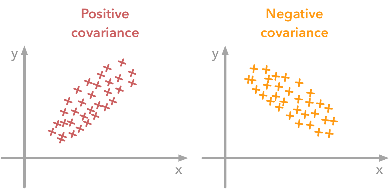
Covariance is the basic quantity for measuring whether two variables tend to deviate from their means in the same direction.

Let

$${\mu }_X=\mathbb{E}[X],{\mu }_Y=\mathbb{E}[Y].$$

The covariance of $X$ and $Y$ is

$$\mathrm{Cov}(X,Y)=\mathbb{E}\left[(X-{\mu }_X)(Y-{\mu }_Y)\right].$$

The product inside this expectation explains the sign:

Position relative to mean	Product	Contribution
$X$ high, $Y$ high	positive	positive covariance
$X$ low, $Y$ low	positive	positive covariance
$X$ high, $Y$ low	negative	negative covariance
$X$ low, $Y$ high	negative	negative covariance

Thus:

• $\mathrm{Cov}(X,Y)>0$: they tend to move together.
• $\mathrm{Cov}(X,Y)<0$: one tends to be high when the other is low.
• $\mathrm{Cov}(X,Y)=0$: there is no linear co-movement captured by covariance.

Covariance of a variable with itself is its variance:

$$\mathrm{Cov}(X,X)=\mathrm{Var}(X).$$

The computational form of covariance

As with variance, expanding the centered expression gives a convenient identity:

$$\mathrm{Cov}(X,Y)=\mathbb{E}[XY]-\mathbb{E}[X]\mathbb{E}[Y].$$

For a discrete joint distribution, calculate $\mathbb{E}[XY]$ by summing over pairs:

$$\mathbb{E}[XY]=\sum _x\sum _{y}xyP(X=x,Y=y).$$

Worked covariance calculation

Let $X$ and $Y$ be binary indicators for two events in a system:

• $X=1$: a request has a high retrieval latency;
• $Y=1$: the request triggers a downstream timeout.

Suppose their joint distribution is:

$X$	$Y$	$P(X,Y)$
$0$	$0$	$0.40$
$0$	$1$	$0.10$
$1$	$0$	$0.10$
$1$	$1$	$0.40$

First, calculate each expectation:

$$\mathbb{E}[X]=P(X=1)=0.10+0.40=\mathrm{0.50.}$$

Similarly,

$$\mathbb{E}[Y]=P(Y=1)=0.10+0.40=\mathrm{0.50.}$$

Because $XY=1$ only when both $X=1$ and $Y=1$,

$$\mathbb{E}[XY]=1(1)(0.40)=\mathrm{0.40.}$$

Now apply the shortcut:

$$\mathrm{Cov}(X,Y)=0.40-(0.50)(0.50)=\mathrm{0.15.}$$

The covariance is positive. High retrieval latency and timeouts occur together more often than they would if the events had no association.

---

Independence, covariance, and variance of sums

For independent variables,

$$\mathrm{Cov}(X,Y)=0.$$

Why? Under independence,

$$\mathbb{E}[XY]=\mathbb{E}[X]\mathbb{E}[Y],$$

so the covariance formula becomes zero.

The reverse statement is not generally true:

$$\mathrm{Cov}(X,Y)=0\nRightarrow X\text{ and }Y\text{ are independent}.$$

For example, let $X$ be uniformly distributed over

$$\{-1,0,1\},$$

and define

$$Y=X^2.$$

Here $Y$ is completely determined by $X$, so the variables are certainly dependent. But symmetry gives

$$\mathbb{E}[X]=0,$$

and

$$\mathbb{E}[XY]=\mathbb{E}[X^3]=0.$$

Therefore,

$$\mathrm{Cov}(X,Y)=0-\mathbb{E}[X]\mathbb{E}[Y]=0.$$

Covariance detects linear association, not every possible dependence pattern. This is especially relevant in feature analysis: a near-zero correlation between two features does not establish that one feature adds no nonlinear information.

Variance of a sum

For any pair of random variables,

$$\mathrm{Var}(X+Y)=\mathrm{Var}(X)+\mathrm{Var}(Y)+2\mathrm{Cov}(X,Y).$$

The covariance term determines how the uncertainties combine:

• Positive covariance makes the total more variable.
• Negative covariance makes the total less variable.
• Independence implies zero covariance, yielding:

$$\mathrm{Var}(X+Y)=\mathrm{Var}(X)+\mathrm{Var}(Y).$$

More generally,

$$\mathrm{Var}(aX+bY)=a^2\mathrm{Var}(X)+b^2\mathrm{Var}(Y)+2ab\mathrm{Cov}(X,Y).$$

This formula is foundational for understanding ensembles, portfolio-style risk calculations, aggregating noisy measurements, and later the covariance matrices used in multivariate ML methods.

---

From distributions to observed datasets

So far, calculations used known probability distributions. In applied ML, we usually have a finite dataset instead.

For observed values $x_1,\dots ,x_n$, the empirical mean is

$$\bar{x}=\frac{1}{n}\sum _{i=1}^n{x}_i.$$

The empirical covariance between features $x$ and $y$ is commonly computed as

$$\widehat{\mathrm{Cov}}(X,Y)=\frac{1}{n-1}\sum _{i=1}^n(x_i-\bar{x})(y_i-\bar{y}).$$

Similarly, the usual sample variance is

$$s^2=\frac{1}{n-1}\sum _{i=1}^n(x_i-\bar{x}{)}^2.$$

The $n-1$ version is the standard unbiased sample estimator of a population variance under common assumptions. In ML code, you may also encounter division by $n$, especially when treating the observed batch or dataset itself as the full population of interest. The key is to state which convention is being used and avoid mixing them silently.

---

Key takeaways

Expectation is the probability-weighted long-run average:

$$\mathbb{E}[X]=\sum _{x}xP(X=x).$$

Variance measures expected squared deviation from the mean:

$$\mathrm{Var}(X)=\mathbb{E}\left[(X-\mathbb{E}[X]{)}^2\right]=\mathbb{E}[X^2]-{\left(\mathbb{E}[X]\right)}^2.$$

Covariance measures whether two variables deviate from their means together:

$$\mathrm{Cov}(X,Y)=\mathbb{E}\left[(X-\mathbb{E}[X])(Y-\mathbb{E}[Y])\right]=\mathbb{E}[XY]-\mathbb{E}[X]\mathbb{E}[Y].$$

Finally, remember the logical distinction:

$$X\text{ and }Y\text{ independent}\Rightarrow \mathrm{Cov}(X,Y)=0,$$

but zero covariance alone does not prove independence.

You have now completed the core mathematical-foundations module. Next, the course moves into statistical reasoning, beginning with how to match common probability distributions—Bernoulli, binomial, Gaussian, and categorical—to modeling situations.