Partial Derivatives and Gradients of Multivariable Functions

Hello. The previous lesson used SVD to describe linear transformations and low-rank structure. We now shift to the calculus used to optimize machine-learning models: how a scalar quantity such as a loss changes when its inputs or parameters change.

This lesson develops two closely related ideas:

• a partial derivative, which measures sensitivity to one input while holding the others fixed;
• a gradient, which collects all of those sensitivities into one vector.

For an ML Engineer interview, be ready to state both the computation and the interpretation: a gradient is not merely “a vector of derivatives”; it is the local direction of steepest increase of a scalar function.

---

Partial derivatives: one coordinate at a time

A single-variable derivative answers: “If $x$ changes slightly, how does $f(x)$ change?”

For a function of two variables,

$$f(x,y),$$

we must specify which coordinate is changing. The partial derivative with respect to $x$, evaluated at $(a,b)$, is

$$\frac{\partial f}{\partial x}(a,b)=\underset{h\to 0}{\lim }\frac{f(a+h,b)-f(a,b)}{h}.$$

Here, $y$ remains fixed at $b$. Similarly,

$$\frac{\partial f}{\partial y}(a,b)=\underset{h\to 0}{\lim }\frac{f(a,b+h)-f(a,b)}{h},$$

where $x$ remains fixed at $a$.

The notation matters:

$$f_x,\frac{\partial f}{\partial x},{\partial }_{x}f$$

all denote the partial derivative with respect to $x$.

The practical rule is simple:

When differentiating with respect to one variable, treat every other independent variable as a constant.

Consider

$$f(x,y)=x^{2}y+3x{y}^2-4y.$$

To find the partial derivative with respect to $x$, treat $y$ as a constant:

$$\frac{\partial f}{\partial x}=2xy+3y^2.$$

The term $-4y$ has no $x$, so it behaves as a constant and vanishes.

To find the partial derivative with respect to $y$, instead treat $x$ as a constant:

$$\frac{\partial f}{\partial y}=x^2+6xy-4.$$

At the point $(1,2)$,

$$\frac{\partial f}{\partial x}(1,2)=2(1)(2)+3(2{)}^2=16,$$

and

$$\frac{\partial f}{\partial y}(1,2)=(1{)}^2+6(1)(2)-4=9.$$

These are local rates of change, not the function value. At $(1,2)$, moving in the positive $x$-direction while keeping $y=2$ fixed increases $f$ at an instantaneous rate of $16$ per unit of $x$. Moving in the positive $y$-direction while keeping $x=1$ fixed increases it at a rate of $9$ per unit of $y$.

---

Partial derivatives as slopes on a surface

For a scalar function of two inputs, $z=f(x,y)$ forms a surface in three-dimensional space. A partial derivative is the slope of a particular cross-section of that surface.

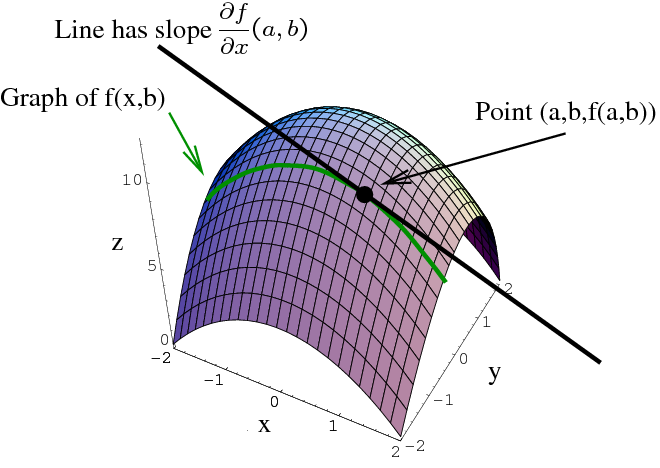
In the image, changing $x$ while holding $y=b$ fixed traces the green curve. That curve is an ordinary one-variable function, so its tangent slope is exactly

$$\frac{\partial f}{\partial x}(a,b).$$

The analogous $y$-slice gives

$$\frac{\partial f}{\partial y}(a,b).$$

This geometric picture is useful, but ML parameter spaces typically have thousands, millions, or billions of coordinates. We cannot visualize their surfaces. Partial derivatives remain meaningful because their definition does not depend on drawing the surface: each one measures what happens when exactly one coordinate changes and the rest are held fixed.

For a scalar function of $n$ variables,

$$f(x_1,x_2,\dots ,x_n),$$

there are $n$ first partial derivatives:

$$\frac{\partial f}{\partial x_1},\frac{\partial f}{\partial x_2},\dots ,\frac{\partial f}{\partial x_n}.$$

For example, if

$$g(a,b,c)=a^{2}b+b{c}^3-4c,$$

then

$$\frac{\partial g}{\partial a}=2ab,$$ $$\frac{\partial g}{\partial b}=a^2+c^3,$$

and

$$\frac{\partial g}{\partial c}=3b{c}^2-4.$$

When differentiating with respect to $c$, both $a^{2}b$ and the coefficient $b$ in $b{c}^3$ are treated as constants.

---

The gradient: all first-order sensitivities together

When the output is scalar, the gradient packages every first partial derivative into a vector:

$$\nabla f(x,y)=\left[\begin{array}{c}\frac{\partial f}{\partial x}(x,y)\\ \frac{\partial f}{\partial y}(x,y)\end{array}\right].$$

For a function of $n$ variables,

$$\nabla f(\mathbf{x})=\left[\begin{array}{c}\frac{\partial f}{\partial x_1}\\ \frac{\partial f}{\partial x_2}\\ ⋮\\ \frac{\partial f}{\partial x_n}\end{array}\right].$$

The symbol $\nabla$ is called nabla or del. In ML literature, gradients are often written as row vectors, but treating them as column vectors makes the shapes in matrix expressions especially clear. The essential requirement is to keep conventions consistent.

For the earlier function,

$$f(x,y)=x^{2}y+3x{y}^2-4y,$$

the gradient is

$$\nabla f(x,y)=\left[\begin{array}{c}2xy+3y^2\\ x^2+6xy-4\end{array}\right].$$

At $(1,2)$,

$$\nabla f(1,2)=\left[\begin{array}{c}16\\ 9\end{array}\right].$$

This says that, locally, $f$ is more sensitive to a small positive change in $x$ than to an equally sized positive change in $y$.

A compact way to express the local behavior of a differentiable function is the first-order approximation:

$$f(\mathbf{p}+\Delta \mathbf{p})\approx f(\mathbf{p})+\nabla f(\mathbf{p}{)}^{\top }\Delta \mathbf{p}.$$

The approximation says: for a sufficiently small input change $\Delta \mathbf{p}$, the change in the function is approximately the dot product of the gradient with that input change.

This connects directly to the dot-product material from earlier in the course. The gradient turns a small vector of coordinate changes into an approximate scalar change in the output.

---

Direction, magnitude, and steepest change

Let $\mathbf{u}$ be a unit vector indicating a direction. The instantaneous rate of change of $f$ in that direction is

$$D_{\mathbf{u}}f(\mathbf{p})=\nabla f(\mathbf{p}{)}^{\top }\mathbf{u}.$$

Using the dot-product identity,

$$\nabla f(\mathbf{p}{)}^{\top }\mathbf{u}=\Vert \nabla f(\mathbf{p})\Vert \Vert \mathbf{u}\Vert \cos \varphi ,$$

and because $\mathbf{u}$ is a unit vector,

$$D_{\mathbf{u}}f(\mathbf{p})=\Vert \nabla f(\mathbf{p})\Vert \cos \varphi .$$

Here, $\varphi$ is the angle between the gradient and the chosen direction.

Three consequences follow immediately:

• The directional derivative is largest when $\mathbf{u}$ points in the same direction as $\nabla f$.
• The maximum rate of increase is

$$\Vert \nabla f(\mathbf{p})\Vert .$$

• The fastest local decrease is in the opposite direction,

$$-\nabla f(\mathbf{p}).$$

A direction perpendicular to the gradient has zero directional derivative:

$$\nabla f(\mathbf{p}{)}^{\top }\mathbf{u}=0.$$

In two dimensions, these are directions tangent to the function's level curves, where the function remains locally constant. The gradient is normal, or perpendicular, to such level curves.

A zero gradient,

$$\nabla f(\mathbf{p})=0,$$

means there is no first-order change in any direction. Such a point is called stationary. It is important not to overinterpret this condition:

• it may be a local minimum;
• it may be a local maximum;
• it may be a saddle point;
• it may occur on a flat region.

For example,

$$s(x,y)=x^2-y^2$$

has

$$\nabla s(x,y)=\left[\begin{array}{c}2x\\ -2y\end{array}\right],$$

so

$$\nabla s(0,0)=0.$$

But $(0,0)$ is neither a minimum nor a maximum: moving along the $x$-axis increases $s$, while moving along the $y$-axis decreases it.

---

Gradients in ML parameter space

In machine learning, the scalar function is usually a loss, objective, or log-likelihood, and the input vector is a parameter vector.

Suppose a model has two parameters:

$$\mathbf{w}=\left[\begin{array}{c}{w}_1\\ w_2\end{array}\right],$$

and, for illustration, its loss is

$$L(w_1,w_2)=(w_1-2{)}^2+3(w_2+1{)}^2.$$

The gradient with respect to the parameters is

$${\nabla }_{\mathbf{w}}L=\left[\begin{array}{c}\frac{\partial L}{\partial w_1}\\ \frac{\partial L}{\partial w_2}\end{array}\right]=\left[\begin{array}{c}2(w_1-2)\\ 6(w_2+1)\end{array}\right].$$

At

$$\mathbf{w}=\left[\begin{array}{c}0\\ 1\end{array}\right],$$

the gradient is

$${\nabla }_{\mathbf{w}}L=\left[\begin{array}{c}-4\\ 12\end{array}\right].$$

Interpret each coordinate carefully:

• $\frac{\partial L}{\partial w_1}=-4$: increasing $w_1$ slightly would locally decrease the loss.
• $\frac{\partial L}{\partial w_2}=12$: increasing $w_2$ slightly would locally increase the loss.

Thus, the gradient identifies a local uphill direction for the loss. Its negative identifies a local downhill direction. The next lesson will formalize how the chain rule lets us compute these gradients through model computations, and how a gradient-based update uses them.

For a neural network, $\mathbf{w}$ may represent every weight and bias in the model. The same definition applies:

$${\nabla }_{\mathbf{w}}L=\left[\begin{array}{c}\frac{\partial L}{\partial w_1}\\ \frac{\partial L}{\partial w_2}\\ ⋮\\ \frac{\partial L}{\partial w_d}\end{array}\right].$$

The dimensionality may be enormous, but each coordinate still answers the same question: How would the scalar loss change if this one parameter changed infinitesimally while all other parameters were fixed?

---

Calculation discipline and common mistakes

When computing gradients by hand, use this reliable sequence:

1. Identify the scalar output. A gradient is defined here for a scalar-valued function such as $L(\mathbf{w})$.
2. Fix the coordinate order. For $f(x,y,z)$, use the order $x,y,z$ consistently.
3. Differentiate symbolically first. Substitute a point only after finding all partial derivatives.
4. Treat non-active variables as constants.
5. Evaluate every component at the same point.
6. Check the resulting gradient shape. It must have one component per input coordinate.

A useful numerical sanity check for the $i$-th gradient component is the central finite-difference approximation:

$$\frac{\partial f}{\partial x_i}(\mathbf{x})\approx \frac{f(\mathbf{x}+ϵ{\mathbf{e}}_i)-f(\mathbf{x}-ϵ{\mathbf{e}}_i)}{2ϵ}.$$

Here, ${\mathbf{e}}_i$ is the vector with a $1$ in coordinate $i$ and zeros elsewhere, and $ϵ$ is small. This is conceptually what gradient checking compares against an analytically derived or automatic-differentiation gradient.

Two distinctions are especially worth retaining:

• A gradient applies to a scalar output. If a function has vector output, its first derivative is generally a Jacobian matrix.
• A gradient is a local, first-order description. It need not predict the effect of a large parameter change, especially on a strongly curved or non-smooth loss surface.

Most ML objectives are differentiable almost everywhere. Some common components, such as the ReLU activation at zero, are not differentiable at isolated points; frameworks select a conventional subgradient there. The standard gradient machinery still applies broadly, but it is useful to know that “a partial derivative exists everywhere” is stronger than practical ML requires.

---

Key takeaways

A partial derivative measures the change in a function as one coordinate varies and all other coordinates remain fixed:

$$\frac{\partial f}{\partial x_i}.$$

The gradient collects every first partial derivative of a scalar function:

$$\nabla f(\mathbf{x})=\left[\begin{array}{c}\frac{\partial f}{\partial x_1}\\ ⋮\\ \frac{\partial f}{\partial x_n}\end{array}\right].$$

It provides the first-order approximation

$$f(\mathbf{x}+\Delta \mathbf{x})\approx f(\mathbf{x})+\nabla f(\mathbf{x}{)}^{\top }\Delta \mathbf{x},$$

points in the direction of maximum local increase, and has magnitude equal to that maximum rate of increase. In an ML loss landscape, each gradient coordinate is the local sensitivity of loss to one parameter.

Next, you will apply the chain rule through a small computational graph and use the resulting gradient in a gradient-descent update—the core calculation underlying backpropagation and training.