Understanding VAEs: Architecture, Objective, and the Reparameterization Trick

Hello! Welcome to the third lesson in our module on the Foundations of Generative Modeling.

In the last lesson, we delved into the architecture of Deep Convolutional Generative Adversarial Networks (DCGANs). We saw how specific architectural guidelines—like using strided convolutions, batch normalization, and particular activation functions—made the adversarial training process more stable and effective, enabling the generation of high-quality images. The core idea remained the adversarial game, where the model learns an implicit data distribution.

Today, we shift our focus to a different family of generative models that takes a more explicitly probabilistic approach. While these models are often introduced with image data, their core principles are fundamental to advanced audio generation models you're interested in, such as the vocoder in VITS.

Your learning outcome for this lesson is to: Explain the architecture and objective function of a Variational Autoencoder (VAE), including the reparameterization trick.

We will dissect the VAE from three perspectives you appreciate: the mathematical theory, the network architecture, and its practical implementation.

1. From Autoencoder to a Generative Model

You are likely familiar with the standard autoencoder from your coursework. It's a neural network trained to reconstruct its input. It consists of:

1. An encoder that compresses the input data $x$ into a low-dimensional latent representation $z$.
2. A decoder that reconstructs the original data $\hat{x}$ from $z$.
   The network is trained to minimize a reconstruction loss, such as Mean Squared Error between $x$ and $\hat{x}$.

However, a standard autoencoder is not a good generative model. Its latent space is often disorganized and non-continuous. If you randomly sample a point $z$ from this latent space and pass it to the decoder, you'll likely get nonsensical output.

To see why, let's watch a brief animation.

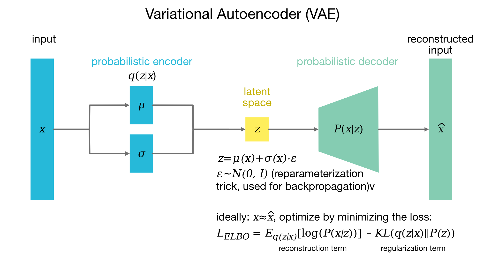
Variational Autoencoders (VAEs) solve this problem by introducing a probabilistic twist. Instead of mapping an input to a single point in the latent space, the VAE encoder maps it to a probability distribution. Specifically, for each input $x$, the encoder outputs the parameters—a mean $\mu$ and a variance ${\sigma }^2$—of a Gaussian distribution. A latent vector $z$ is then sampled from this distribution.

This simple change has a profound effect:

• It forces the latent space to be continuous and smoothly organized.
• It allows us to frame the entire model in a rigorous probabilistic way, giving us a clear objective function to optimize.

The overall architecture looks like this:

2. The Probabilistic Framework and the ELBO

Since you're interested in the underlying math, let's build the VAE from first principles.

A VAE is a probabilistic generative model. We assume our data $x$ is generated from some latent variable $z$. The generative process is:

1. Sample a latent vector $z$ from a simple prior distribution, $p(z)$. Typically, this is a standard multivariate normal distribution, $p(z)=\mathcal{N}(0,I)$.
2. Generate the data point $x$ by sampling from a conditional distribution $p_{\theta }(x|z)$. This distribution is parameterized by a complex function (the decoder neural network with parameters $\theta$) that maps $z$ to the parameters of the output distribution.

Our goal is to find the parameters $\theta$ that maximize the likelihood of our observed data, $p(x)$. The likelihood of a single data point is given by marginalizing over the latent variables:

$$p(x)=\int p_{\theta }(x|z)p(z)dz$$

This integral is intractable because it requires integrating over all possible values of $z$, which is computationally infeasible for a high-dimensional latent space and a complex decoder.

The Evidence Lower Bound (ELBO)

To handle this, we introduce an inference model (the encoder), denoted $q_{\varphi }(z|x)$, with parameters $\varphi$. This network's job is to approximate the true but intractable posterior distribution $p_{\theta }(z|x)$.

Now, we can decompose the log-likelihood of our data, $\log p(x)$, as follows. Since the expectation of a constant is the constant itself, we can write:

$$\log p(x)={\mathbb{E}}_{z\sim q_{\varphi }(z|x)}[\log p(x)]$$

Using the definition of conditional probability, $p(x)=\frac{p_{\theta }(x,z)}{p_{\theta }(z|x)}$, and introducing $q_{\varphi }(z|x)$ in the numerator and denominator:

$$\log p(x)={\mathbb{E}}_{z\sim q_{\varphi }(z|x)}\left[\log \left(\frac{p_{\theta }(x,z)}{q_{\varphi }(z|x)}\frac{q_{\varphi }(z|x)}{p_{\theta }(z|x)}\right)\right]$$

Splitting the logarithm:

$$\log p(x)={\mathbb{E}}_{z\sim q_{\varphi }(z|x)}\left[\log \left(\frac{p_{\theta }(x,z)}{q_{\varphi }(z|x)}\right)\right]+{\mathbb{E}}_{z\sim q_{\varphi }(z|x)}\left[\log \left(\frac{q_{\varphi }(z|x)}{p_{\theta }(z|x)}\right)\right]$$

This gives us our final, crucial relationship:

$$\log p(x)=\underset{\text{ELBO}}{\underbrace{\mathcal{L}(\theta ,\varphi ;x)}}+\underset{\text{KL Divergence}}{\underbrace{D_{KL}(q_{\varphi }(z|x)||p_{\theta }(z|x))}}$$

The first term, $\mathcal{L}(\theta ,\varphi ;x)$, is the Evidence Lower Bound (ELBO). The second term is the Kullback-Leibler (KL) divergence between our approximate posterior and the true posterior. Since KL divergence is always non-negative ($D_{KL}\ge 0$), the ELBO is a lower bound on the log-likelihood of the data.

By maximizing the ELBO, we are simultaneously:

1. Pushing up the lower bound on the data likelihood, thus training our generative model.
2. Minimizing the KL divergence between our encoder's approximation and the true posterior, thus training our inference model.

Deconstructing the ELBO

The ELBO itself can be rewritten into a more intuitive form:

$$\mathcal{L}(\theta ,\varphi ;x)={\mathbb{E}}_{z\sim q_{\varphi }(z|x)}[\log p_{\theta }(x|z)]-D_{KL}(q_{\varphi }(z|x)||p(z))$$

This form reveals the two core components of the VAE's objective function (when framed as a loss function to be minimized, we just negate the ELBO):

1. Reconstruction Loss: The first term, $-{\mathbb{E}}_{z\sim q_{\varphi }(z|x)}[\log p_{\theta }(x|z)]$, measures how well the decoder can reconstruct the input $x$ given a latent sample $z$ from the encoder. If the decoder $p_{\theta }(x|z)$ is assumed to be a Gaussian distribution, this term becomes equivalent to minimizing the mean squared error between the input $x$ and the reconstructed output $\hat{x}$.

2. KL Divergence (Regularization): The second term, $D_{KL}(q_{\varphi }(z|x)||p(z))$, acts as a regularizer. It measures the "distance" between the distribution produced by the encoder for a given input $x$ and the prior distribution $p(z)$. It forces the encoder to learn distributions that are close to a standard normal, which organizes the latent space and makes it suitable for generation.

Let's watch a video that visualizes this objective and its components.

For a deeper dive into the mathematics, the following resources provide full derivations of both the ELBO and the analytical formula for the KL divergence term when both distributions are Gaussian.

3. Making it Trainable: The Reparameterization Trick

We have a clear objective function, but there's a major roadblock. The expectation term ${\mathbb{E}}_{z\sim q_{\varphi }(z|x)}$ involves a sampling step. How can we backpropagate gradients through a random sampling operation to train the encoder's parameters $\varphi$?

This is where the reparameterization trick comes in.

The trick is to re-express the random variable $z$ in a way that separates the randomness from the network parameters. Instead of directly sampling $z$ from the distribution defined by the encoder, $z\sim \mathcal{N}({\mu }_{\varphi }(x),{\sigma }_{\varphi }^2(x))$, we do the following:

1. Sample a random noise vector $ϵ$ from a standard normal distribution, $ϵ\sim \mathcal{N}(0,I)$. This sampling is external to the network and has no parameters to train.
2. Compute $z$ as a deterministic function of $\mu$, $\sigma$, and $ϵ$: $$z={\mu }_{\varphi }(x)+{\sigma }_{\varphi }(x)\odot ϵ$$ where $\odot$ denotes element-wise multiplication.

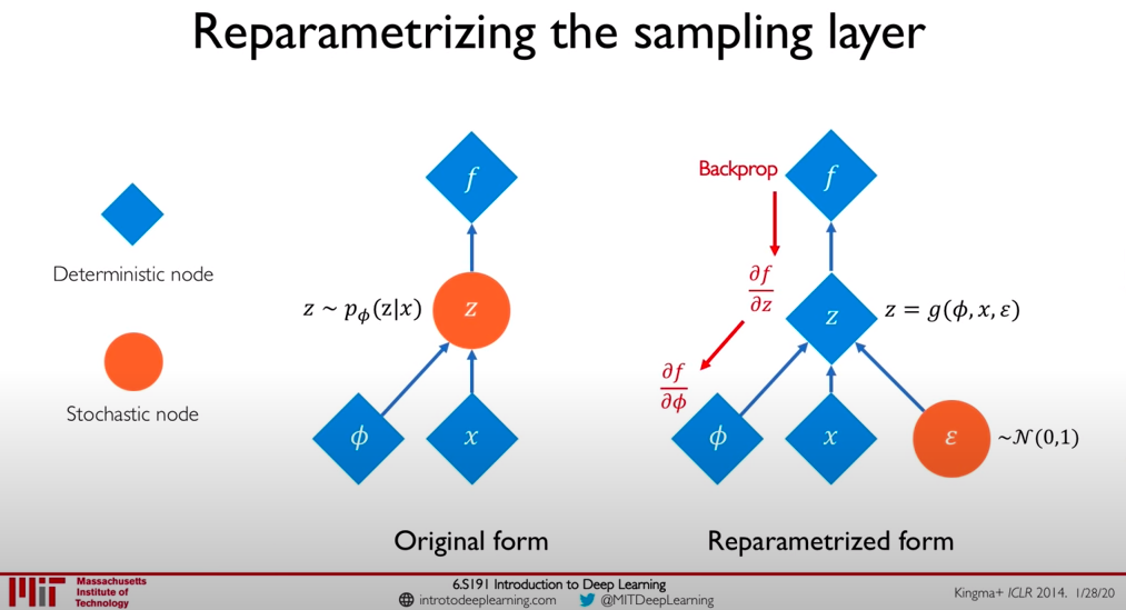
Now, the stochasticity is isolated in $ϵ$, while the path from the encoder parameters $\varphi$ (which produce $\mu$ and $\sigma$) to $z$ is fully deterministic and differentiable. This allows us to use standard backpropagation to train the entire VAE end-to-end.

This animation and a deeper lecture segment will solidify the concept.

4. The VAE in Practice

Let's consolidate the architecture and training process with a look at a code implementation. The forward pass of a VAE and its loss function can be implemented in PyTorch as follows:

The full process for a single data point $x$ is:

1. Encode: Pass $x$ through the encoder to get $\mu$ and $\log ({\sigma }^2)$.
2. Reparameterize: Sample $ϵ\sim \mathcal{N}(0,I)$ and compute $z=\mu +\exp (0.5\cdot \log ({\sigma }^2))\cdot ϵ$.
3. Decode: Pass $z$ through the decoder to get the reconstruction $\hat{x}$.
4. Calculate Loss: Compute the total loss as the sum of the reconstruction loss (e.g., MSE between $x$ and $\hat{x}$) and the KL divergence term, which can be calculated analytically from $\mu$ and ${\sigma }^2$.
5. Backpropagate: Compute gradients and update the parameters $\theta$ and $\varphi$ of the decoder and encoder.

Conclusion

In this lesson, you've learned about Variational Autoencoders, a powerful class of generative models built on the principles of variational inference.

Key Takeaways:

• Architecture: A VAE consists of a probabilistic encoder $q_{\varphi }(z|x)$ that maps an input to a distribution in the latent space (typically a Gaussian defined by $\mu$ and ${\sigma }^2$), and a probabilistic decoder $p_{\theta }(x|z)$ that reconstructs the input from a latent sample.
• Objective Function: VAEs are trained by maximizing the Evidence Lower Bound (ELBO), which is equivalent to minimizing a loss function composed of two terms: a reconstruction loss that ensures fidelity and a KL divergence term that regularizes the latent space.
• The Reparameterization Trick: This crucial technique allows gradients to be backpropagated through the stochastic sampling step by reformulating the latent variable $z$ as a deterministic function of the encoder's outputs and a parameter-free noise variable $ϵ$.

Preview of the Next Lesson:

We have now studied two major families of generative models: GANs and VAEs. While both learn to generate data, they do so in fundamentally different ways, which results in distinct characteristics in their learned latent spaces. In the next lesson, we will distinguish between the latent spaces learned by GANs and VAEs, comparing their structure, continuity, and how they can be manipulated. We will also briefly introduce a third generative model family, Normalizing Flows, which offer another distinct approach to modeling complex distributions.