Introduction to Normalizing Flows

Hello! Welcome to the fifth lesson in our module on the Foundations of Generative Modeling.

In the previous lessons, we explored the landscapes of Generative Adversarial Networks (GANs) and Variational Autoencoders (VAEs). We saw how VAEs optimize a lower bound on the data likelihood, giving us a structured latent space at the cost of sample sharpness. We also saw how GANs bypass likelihood entirely to achieve incredible realism, but with challenges in training stability and latent space control.

You now understand the core trade-offs between these two major families. Today, we introduce a third, powerful approach that addresses a key limitation of both: Normalizing Flows. These models offer a way to compute the exact data log-likelihood while maintaining a direct, invertible mapping between the data and latent space. This is a crucial concept, as components of advanced audio models like VITS use flows to transform distributions.

Your learning outcome for this lesson is to: Describe the concept of Normalizing Flows for constructing complex probability distributions from simple ones.

We will unpack the elegant mathematical principle that allows these models to "flow" from a simple, easy-to-sample distribution (like a Gaussian) to a complex one that matches your data.

1. The Core Idea: Transforming Probability Distributions

Imagine you have a large pile of sand representing a simple, known probability distribution, like a standard normal (Gaussian) distribution. Now, imagine you carefully sculpt that sand into an intricate castle. The sand castle represents the complex, high-dimensional distribution of your real-world data (e.g., all possible human speech).

Normalizing Flows formalize this idea. They learn a series of invertible and differentiable transformations that morph a simple base distribution, $p_z(\mathbf{z})$, into a target distribution, $p_x(\mathbf{x})$, that matches the data.

The key to making this work lies in a fundamental rule of probability theory: the change of variables theorem.

2. The Mathematics: Change of Variables

When you transform a random variable, its probability density function also changes. If you stretch a region of space, the probability density in that region must decrease to ensure the total probability remains 1. Conversely, if you compress a region, the density must increase.

The change of variables theorem gives us the exact formula to calculate the new density.

• For a single variable: If we have a variable $z$ with density $p_z(z)$ and an invertible function $x=f(z)$, the density of the new variable $x$, $p_x(x)$, is given by:

  $$p_x(x)=p_z(f^{-1}(x))\left|\frac{d{f}^{-1}(x)}{dx}\right|$$

  The term $\left|\frac{d{f}^{-1}(x)}{dx}\right|$ is the scaling factor that accounts for the stretching or compressing of the space.

• For multiple variables: This extends to vectors $\mathbf{z}$ and $\mathbf{x}$. The scaling factor becomes the absolute value of the determinant of the Jacobian matrix of the transformation. The Jacobian matrix contains all the first-order partial derivatives of the function and its determinant measures how much a local volume of space expands or contracts.

  $$p_x(\mathbf{x})=p_z(f^{-1}(\mathbf{x}))\left|\det \left(\frac{\partial f^{-1}(\mathbf{x})}{\partial \mathbf{x}}\right)\right|$$

  where $\frac{\partial f^{-1}(\mathbf{x})}{\partial \mathbf{x}}$ is the Jacobian of the inverse function $f^{-1}$.

To build a solid intuition for this crucial theorem, the following video provides an excellent step-by-step derivation, starting from the 1D case and building up to the multi-dimensional formula.

Because we often work with log-probabilities for numerical stability, we can write the log-likelihood as:

This equation is the heart of Normalizing Flows. It tells us that if we can compute the inverse of our transformation $f$ and the determinant of its Jacobian, we can calculate the exact log-likelihood of any data point $\mathbf{x}$. This is a significant advantage over VAEs and GANs.

3. Stacking Transformations: The "Flow"

A single simple transformation is not powerful enough to model a complex data distribution. The main insight of Normalizing Flows is to compose or chain a sequence of simpler invertible transformations.

Let's say we have a sequence of $K$ invertible functions $f_1,f_2,...,f_K$.
We start with a sample ${\mathbf{z}}_0$ from our simple base distribution $p_0({\mathbf{z}}_0)$.

The full transformation is $\mathbf{x}=f_K\circ \cdots \circ f_1({\mathbf{z}}_0)$. Since the composition of invertible functions is itself invertible, we can still apply the change of variables rule.

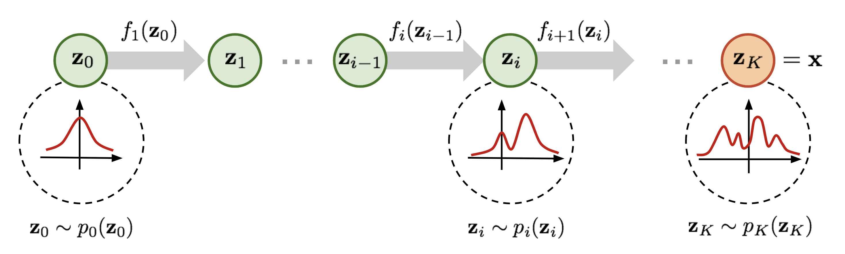
Applying the log-likelihood formula recursively, we find that the log-determinant of the full transformation is simply the sum of the log-determinants of each individual transformation. This is because $\det (AB)=\det (A)\det (B)$, so $\log \det (AB)=\log \det (A)+\log \det (B)$.

This gives us the final log-likelihood objective for a Normalizing Flow:

Or, using an equivalent formulation with the forward Jacobian:

This is the objective function we maximize during training. To see the derivation laid out clearly, I recommend the following resource.

4. The Normalizing Flow Recipe

To build a practical Normalizing Flow model, the transformations $f_i$ must satisfy two crucial properties:

1. They must be easily invertible. For training, we need to go from data to latent ($\mathbf{x}\to {\mathbf{z}}_0$) to compute the likelihood. For generation, we need to go from latent to data (${\mathbf{z}}_0\to \mathbf{x}$).
2. The determinant of their Jacobian must be easy and efficient to compute. A naive calculation of a determinant for a $D\times D$ matrix is $O(D^3)$, which is intractable for high-dimensional data like audio or images. We need transformations whose Jacobian has a special structure (e.g., triangular or diagonal), making the determinant calculation $O(D)$.

The main research in Normalizing Flows focuses on designing neural network layers that satisfy these two constraints while being expressive enough to model complex data.

In the next lesson, we will explore specific examples of these transformations, such as affine coupling layers used in models like RealNVP and Glow. These clever designs ensure the Jacobian matrix is triangular, making its determinant simply the product of the diagonal elements, thus satisfying the efficiency constraint.

To get a first glimpse of how this works, the following short video segment introduces the idea.

Conclusion

You have now learned the fundamental concept behind Normalizing Flows. Unlike VAEs that optimize a bound or GANs that discard likelihood, flows provide a method for exact likelihood estimation through a series of invertible transformations.

Key Takeaways:

• Normalizing Flows construct complex distributions by applying a sequence of invertible transformations to a simple base distribution.
• The Change of Variables theorem is the mathematical foundation, relating the probability densities of the original and transformed variables via the Jacobian determinant.
• This framework allows for exact and tractable computation of the log-likelihood of the data, which is used as the training objective.
• The key design challenge is creating transformations that are both expressive and computationally efficient, meaning they are easy to invert and their Jacobian determinant is fast to compute.

Preview of the Next Lesson:

We've covered the "what" and "why" of Normalizing Flows. In the next lesson, we'll dive into the "how." We will explore the ingenious designs of invertible transformations, such as coupling and autoregressive layers, that satisfy the necessary constraints and make Normalizing Flows practical and powerful generative models.