GANs, VAEs, and Flow-based Models: A Comparative Analysis

Hello! Welcome back to the final lesson in our module on the foundations of generative modeling.

In the previous lessons, we've dissected the three major families of deep generative models. We saw how:

Variational Autoencoders (VAEs) learn a data distribution by maximizing a lower bound on the log-likelihood (the ELBO).
Generative Adversarial Networks (GANs) learn through a competitive game between a generator and a discriminator, without an explicit likelihood objective.
Normalizing Flows learn an exact likelihood by transforming a simple distribution into a complex one through a series of invertible functions.

Now that we understand the core mechanics of each, it's time to put them side-by-side. Your learning outcome for this lesson is to compare and contrast the characteristics of GANs, VAEs, and Flow-based models in terms of sample quality, diversity, and training stability. This comparative understanding is crucial for selecting, designing, and troubleshooting generative models for audio and other domains.

1. A Framework for Comparison

At a high level, all three models aim to learn a distribution $p (x)$ but go about it in fundamentally different ways. The image below, which you may recognize from one of our resources, neatly summarizes the architectural and objective differences.

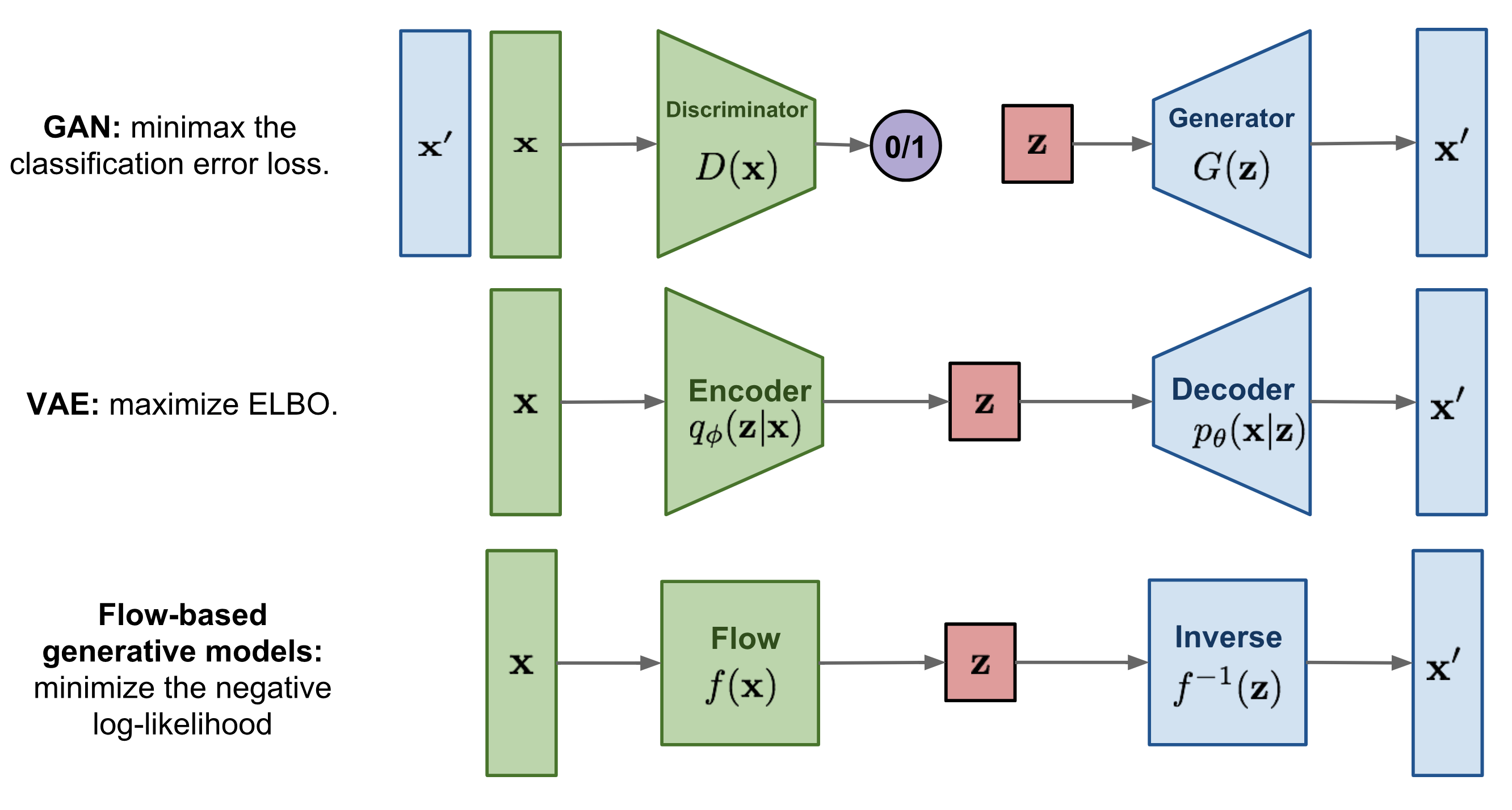
Comparison of Generative Adversarial Networks (GANs), Variational Autoencoders (VAEs), and Flow-based Generative Models — A high-level overview of GANs, VAEs, and Flow-based models. Each has a distinct architecture and optimization objective, leading to different strengths and weaknesses. Source: Lilian Weng, "Flow-based Deep Generative Models".

To structure our comparison, we will evaluate these models against a set of key characteristics that are critical in practice:

Training Objective & Stability: What is being optimized, and how reliable is the training process?
Sample Quality: How realistic are the generated samples?
Sample Diversity (Mode Coverage): Does the model capture the full variety of the data, or does it miss or ignore certain modes?
Likelihood Calculation: Can the model compute the exact probability $p (x)$ for a given data point?
Latent Space: Is there an efficient way to get a latent representation $z$ from a data point $x$ , and is this latent space useful for tasks like interpolation?

Let's start by reinforcing the key theoretical differences in how these models handle likelihood and inference.

What are Normalizing Flows?

The following clip from the video "What are Normalizing Flows?" by Ari Seff directly contrasts the three model families based on their approach to likelihood and posterior inference.

Please watch from 4:29 to 6:48. Focus on how the video explains the differences between Normalizing Flows, VAEs, and GANs regarding: Likelihood Evaluation: Which models compute an exact likelihood, which compute an approximation (a bound), and which avoid it entirely? Posterior Inference: How does each model handle the task of finding the latent code z that corresponds to a given data point x?

2. The Core Trade-offs: Quality, Diversity, and Stability

The different training objectives you just reviewed lead directly to the central trade-offs between these models.

Generative Adversarial Networks (GANs)

Training: The adversarial, minimax objective is notoriously unstable. It requires careful balancing of the generator and discriminator, and training can fail to converge. It often suffers from vanishing gradients or mode collapse.
Sample Quality: This is where GANs have historically shined. The adversarial loss acts as a highly adaptive perceptual loss function, pushing the generator to produce extremely sharp and realistic samples to fool the discriminator.
Sample Diversity: GANs are highly susceptible to mode collapse. The generator might find a few "tricks" (modes) that consistently fool the discriminator and overproduce samples from those modes while ignoring others. This results in low sample diversity.
Likelihood & Latent Space: GANs do not learn an explicit density function, so calculating $p (x)$ is intractable. Standard GANs also lack an encoder, making inference (mapping $x \to z$ ) difficult.

Variational Autoencoders (VAEs)

Training: Training is very stable as it involves optimizing a single, well-defined loss function (the ELBO).
Sample Quality: Samples from basic VAEs are often perceived as blurry or overly smooth. This is often attributed to the pixel-wise reconstruction loss (like MSE) and the limitations of the Gaussian posterior assumption.
Sample Diversity: VAEs generally exhibit good mode coverage. The reconstruction term in the ELBO forces the model to be able to encode and decode all samples in the dataset, discouraging it from ignoring modes.
Likelihood & Latent Space: VAEs provide a lower bound (the ELBO) on the likelihood, not the exact value. They have an explicit encoder, making inference ( $x \to z$ ) fast and efficient. The latent space is often smooth and continuous, making it well-suited for interpolation.

Flow-based Models

Training: Like VAEs, training is very stable as it directly optimizes the exact negative log-likelihood (NLL).
Sample Quality: Sample quality is often good but can sometimes lag behind the best GANs in terms of fine detail and realism.
Sample Diversity: They have excellent mode coverage. Because they are trained with maximum likelihood, they are incentivized to account for the entire data distribution, effectively preventing mode collapse.
Likelihood & Latent Space: This is their biggest strength. They provide exact, tractable likelihoods. The transformation is invertible by design, so inference ( $x \to z$ ) is as efficient as generation.

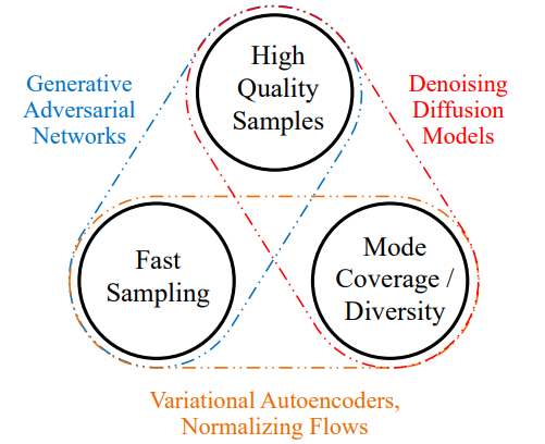
The following visual neatly summarizes these primary trade-offs, and importantly, introduces a fourth category—Denoising Diffusion Models—which we will discuss shortly.

Comparison of Generative Models by Key Characteristics — A diagram illustrating the trade-offs between GANs, VAEs/Flows, and Denoising Diffusion Models in terms of sample quality, sampling speed, and mode coverage/diversity. Notice how each family occupies a different region, highlighting their unique strengths.

3. A Deeper Comparative Review

To add more quantitative rigor to our comparison, we will turn to a comprehensive review paper that benchmarks these models.

First, a quick word on evaluation metrics.

Fréchet Inception Distance (FID): This is a popular metric for measuring the quality and diversity of generated images. It compares the statistics of features from a pre-trained network (InceptionV3) for real and generated images. A lower FID is better.
Negative Log-Likelihood (NLL): For models that can compute it, this measures how well the model's distribution fits a test dataset, often reported in bits-per-dimension (BPD). A lower NLL/BPD is better, indicating a better fit and higher diversity.

Now, let's dive into the data.

Deep Generative Modelling: A Comparative Review

The paper "Deep Generative Modelling: A Comparative Review" provides a fantastic, detailed comparison of generative models. We will focus on the summary table and the sections explaining the pros and cons of each family.

Please read the following parts of the paper: Section 1 (Introduction) and Table 1: Study Table 1 carefully. This is the core of our comparison. Understand what each column represents (Train/Sample Speed, Params, Resolution, FID, NLL). Use Table 2 to understand the star ratings. Skim the text in Section 3 (VAEs), Section 4 (GANs), and Section 6 (Normalizing Flows): You don't need to read every word. Focus on the discussions of common problems and advantages for each model type, such as blurry samples in VAEs (Sec. 3), training instability and mode collapse in GANs (Sec. 4.1), and architectural restrictions in Flows (Sec. 6).

After reviewing the paper, let's consolidate our findings. The table below summarizes the key distinctions we've discussed.

Feature	Generative Adversarial Networks (GANs)	Variational Autoencoders (VAEs)	Flow-based Models
Primary Strength	High-fidelity, sharp sample quality	Stable training, useful latent space for encoding	Exact likelihood evaluation, excellent diversity
Primary Weakness	Training instability, mode collapse	Blurry or overly smooth samples	Restrictive architectural constraints
Training Stability	Low: Unstable minimax game, hard to converge.	High: Stable, single loss function (ELBO).	High: Stable, single loss function (NLL).
Sample Quality	High: Often state-of-the-art.	Medium: Can be blurry without advanced architectures.	High: Competitive, but can lack fine details.
Sample Diversity	Low: Prone to mode collapse.	High: Good mode coverage.	High: Excellent mode coverage.
Likelihood	Intractable: No explicit density model.	Approximate: Computes a lower bound (ELBO).	Exact: The core feature of the model.
Inference ( $x \to z$ )	Hard: No encoder; requires optimization or a separate network.	Easy: Built-in encoder.	Easy: Inverse of the generative function.
Sampling Speed	Fast: Single forward pass.	Fast: Single forward pass.	Varies: Fast for coupling, slow for autoregressive.
Architecture	Flexible: Few constraints on generator/discriminator networks.	Flexible: Few constraints on encoder/decoder networks.	Restrictive: Must be invertible with tractable Jacobian.

4. A Modern Perspective: Score-Based and Diffusion Models

As you saw in the Venn diagram, the field has evolved. The sharp lines between these models have started to blur, with hybrid approaches and new model families emerging. The most significant recent development is the rise of score-based generative models, also known as denoising diffusion probabilistic models (DDPMs).

These models, which you'll notice dominate the top performance spots in Table 1 of the review paper, combine ideas from the families we've studied. They are trained with a stable objective related to score matching (similar to Flows/VAEs) but have been shown to surpass GANs in sample quality. Their main drawback has been slow sampling speed, although recent research is rapidly closing this gap.

For your goal of becoming an audio researcher, understanding these modern models is essential. The following resource provides an expert-level comparison that includes this new family.

Diffusion and Score-Based Generative Models

In this final segment from the MIT lecture on score-based models, the speaker, Dr. Yang Song, directly answers audience questions comparing diffusion models to GANs and VAEs. This is a research-level perspective on the very trade-offs we are discussing.

Please watch the Q&A section from 1:16:39 to 1:22:22. The speaker addresses key questions: Why do diffusion models outperform GANs in sample quality? In what cases do they underperform (e.g., sampling speed)? How do their latent spaces compare?

As Dr. Song highlights, the flexibility of the neural network architecture in diffusion models (enabled by a stable, score-based objective) is a key reason for their superior performance. They effectively achieve the sample quality of GANs while maintaining the training stability and diversity of likelihood-based models, albeit at the cost of sampling speed.

Conclusion

You have now completed your foundational tour of deep generative models. We have moved from the basic principles of VAEs, GANs, and Flows to a nuanced, comparative analysis of their practical strengths and weaknesses.

Key Takeaways:

There is no single "best" generative model; there are fundamental trade-offs between sample quality, sample diversity, and training stability.
GANs are the go-to for top-tier sample quality if you can manage their training instability and potential for mode collapse.
VAEs offer stable training and a meaningful latent space, making them excellent for tasks requiring encoding and interpolation, but may sacrifice some sample fidelity.
Normalizing Flows provide mathematically elegant, stable training and exact density estimation, making them ideal for anomaly detection or scientific modeling, but are architecturally constrained.
Modern approaches like Diffusion Models are changing the landscape by achieving GAN-level quality with the training stability of likelihood-based methods, creating a new set of trade-offs centered on sampling speed.

Preview of the Next Module:

With this solid foundation in generative modeling, you are now well-prepared to tackle specific, large-scale audio models. In our next module, Supervised Speech Recognition Models, we will pivot from generation to transcription. We will begin by formulating speech recognition as a sequence-to-sequence problem and deriving the Connectionist Temporal Classification (CTC) loss function, a cornerstone of modern Automatic Speech Recognition (ASR) systems.