Classifier-Free Guidance for Conditional Image Generation

Hello and welcome back!

In our previous lesson, we assembled the complete architecture for a Latent Diffusion Model (LDM). We saw how it efficiently operates in a compressed latent space and, crucially, how its U-Net is equipped with cross-attention layers. These layers are designed to accept external conditioning information, and we left them waiting for an input. Today, we'll connect that input and unlock the model's text-to-image capabilities.

Your learning outcome for this lesson is to apply classifier-free guidance for conditional image generation. This is the clever and surprisingly simple technique that allows us to steer the powerful but random diffusion process to create images that precisely match a text prompt.

We'll cover:

The core intuition behind "guiding" a diffusion model's denoising path.
The formal mechanism of Classifier-Free Guidance (CFG), including the training trick that makes it possible.
How to implement CFG in a practical sampling pipeline.
The concept of negative prompts as a powerful extension of CFG.

By the end of this lesson, you will have a complete conceptual and practical understanding of how a Latent Diffusion Model becomes a controllable text-to-image generator like Stable Diffusion.

1. The Intuition: Steering the Denoising Process

Imagine the denoising process as a particle moving through a high-dimensional space. At each step, the U-Net tells the particle which way to go to become less noisy. An unconditional model has learned a general direction towards "a realistic image." But how do we tell it to move towards "a realistic image of an astronaut riding a horse"?

The key idea is to give the model two directions at each step:

The direction towards an unconditional, generic image.
The direction towards an image that matches our prompt.

By taking the difference between these two directions, we get a vector that points purely in the "direction of our prompt." We can then amplify this "guidance vector" and add it to the unconditional path, effectively steering the process.

This concept is explained beautifully in the following video.

But how do AI images and videos actually work? | Guest video by Welch Labs

To build a strong visual intuition for classifier-free guidance, let's watch this segment from a video by 3Blue1Brown and Welch Labs. It uses a 2D analogy to make the high-dimensional process easy to grasp.

Watch the section on classifier-free guidance from 28:12 to 34:04. Pay close attention to: The visualization of the unconditional (gray) and conditional (yellow) vector fields. How subtracting the unconditional vector from the conditional one creates a guidance vector. The role of the scaling factor, alpha (often called the guidance scale), in amplifying this direction and how it impacts the final image.

As the video shows, this guidance mechanism is incredibly powerful. The guidance scale (w, or alpha in the video) becomes a hyperparameter that lets us trade diversity for prompt-adherence. A low value gives the model more creative freedom, while a high value forces it to follow the prompt more strictly.

2. The Theory: From Classifier Guidance to Classifier-Free

The idea of steering a diffusion model didn't start with CFG. Its precursor was Classifier Guidance.

Classifier Guidance

The original approach involved using two separate models:

A standard diffusion model.
An image classifier (e.g., ResNet) trained to predict the class of a noisy image.

During sampling, at each step, the classifier would analyze the noisy image $x_{t}$ and calculate a gradient that "pushes" the image towards the desired class (e.g., 'dog'). This gradient was then used to nudge the diffusion model's prediction.

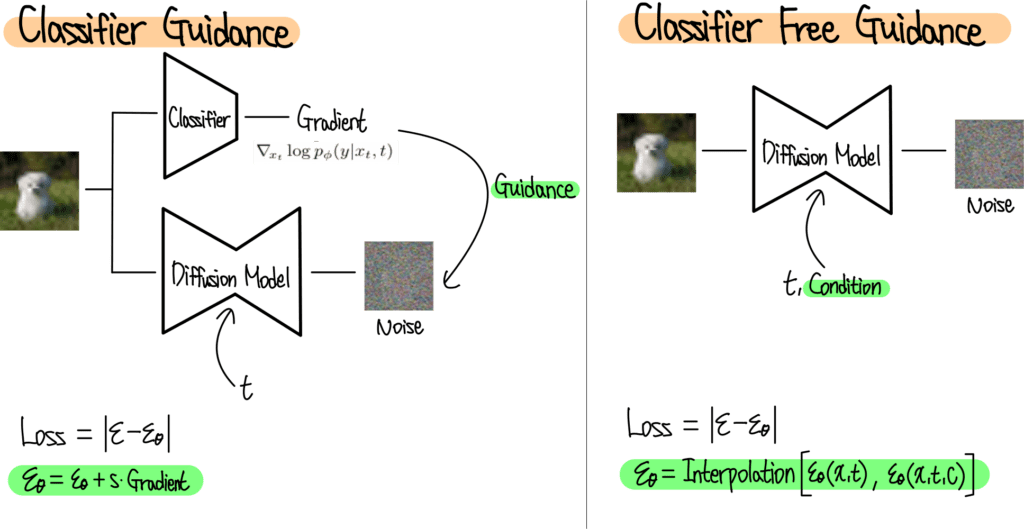
Comparison of Classifier Guidance and Classifier-Free Guidance — This diagram illustrates the two guidance methods. **Left (Classifier Guidance):** A separate classifier model provides an external gradient to steer the diffusion model. **Right (Classifier-Free Guidance):** A single diffusion model, trained to be both conditional and unconditional, provides its own guidance by interpolating between its two modes of prediction.

While effective, this approach was cumbersome. It required training and maintaining a second, noise-aware classifier, which was computationally expensive and complex.

Classifier-Free Guidance (CFG)

In 2021, researchers Jonathan Ho and Tim Salimans proposed a more elegant solution that achieved the same goal without needing a separate classifier. This is the core idea of Classifier-Free Guidance.

An overview of classifier-free guidance for diffusion models

This article from The AI Summer provides a clear theoretical breakdown of both classifier guidance and classifier-free guidance. Let's focus on the sections explaining the transition between the two.

Please read the following two sections: Classifier guidance: Understand how an external classifier and Bayes' rule are used to create a conditional score. Note its main limitation: needing a separate, noise-aware classifier. Classifier-free guidance: This is the key part. Focus on how it reformulates the guidance equation to use a single model. Pay close attention to the conditioning dropout training trick and the final guidance formula.

Let's crystallize the two key innovations of CFG:

Training with Conditioning Dropout: A single U-Net is trained on image-text pairs. However, for a small fraction of the training steps (e.g., 10-20%), the text conditioning is deliberately omitted and replaced with a null or empty token. This forces the same model to learn how to make both conditional predictions (when the prompt is present) and unconditional predictions (when it's absent).
Guidance via Interpolation: During inference, we leverage this dual capability. For each denoising step, we run the U-Net twice in parallel:
- Once with the text prompt c to get the conditional noise prediction, $ϵ_{θ} (z_{t}, c)$ .
- Once with the null token ∅ to get the unconditional noise prediction, $ϵ_{θ} (z_{t}, \emptyset)$ .
We then combine them using a linear interpolation formula to get the final guided noise prediction, $\tilde{ϵ}_{θ}$ :
$\tilde{ϵ}_{θ} (z_{t}, c) = ϵ_{θ} (z_{t}, \emptyset) + w \cdot (ϵ_{θ} (z_{t}, c) - ϵ_{θ} (z_{t}, \emptyset))$
Here, $w$ is the guidance scale (or cfg_scale).
- If $w = 0$ , the guided prediction is just the unconditional one.
- If $w = 1$ , the guided prediction is the purely conditional one.
- If $w > 1$ , we are extrapolating in the direction of the prompt, pushing the model to adhere more strongly to the conditioning. Typical values for Stable Diffusion are between 7 and 12.

Test your understanding!

In the CFG formula above, what does the term $(ϵ_{θ} (z_{t}, c) - ϵ_{θ} (z_{t}, \emptyset))$ represent conceptually? Why is it the core of the guidance mechanism?

Show answer

This term represents the "guidance vector" or the direction in the noise space that points from the unconditional prediction towards the conditional one. It isolates the influence of the prompt c. By scaling this vector with w, we can control how strongly we want to steer the denoising process towards the prompt's semantics, effectively trading off diversity for fidelity.

3. Implementation in Practice

With a solid grasp of the theory, let's see how this is implemented. Since you're familiar with Python and PyTorch, connecting the formula to the code will be straightforward.

Training Modification

First, how do we implement conditioning dropout during training? It's as simple as it sounds.

Diffusion Models | PyTorch Implementation

The 'Diffusion Models | PyTorch Implementation' video by Outlier provides a concise demonstration of the necessary changes for CFG.

Watch the following segments: Model Changes (16:43 - 17:43): See how the model is modified to accept a conditional input (in this case, class labels) by adding an embedding for them to the time step embedding. For Stable Diffusion, this conditioning comes from the CLIP text encoder and is fed into the U-Net's cross-attention layers. Training Loop Changes (17:53 - 18:51): Observe the simple but crucial logic: for a small percentage of training batches, the labels are set to None. This is the conditioning dropout that teaches the model to make unconditional predictions.

Sampling Pipeline

The more interesting part is the sampling loop. You're already familiar with the generate function from the Implementing Stable Diffusion from Scratch article we used in the last lesson. Now, we can finally understand the do_cfg block within it.

Implementing Stable Diffusion from Scratch using PyTorch

Let's revisit the article by Ebad Sayed. The generate function contains a clear implementation of the CFG logic during inference.

Carefully examine the code within the generate function, focusing on the parts related to do_cfg: Context Preparation: Notice how cond_context is generated from the prompt and uncond_context is generated from the uncond_prompt (which is often an empty string). These are then concatenated into a single context tensor. Input Duplication: Inside the main for loop, see the line model_input = model_input.repeat(2, 1, 1, 1). This duplicates the noisy latent z_t to create a batch of size 2, so we can feed both the conditional and unconditional contexts to the U-Net in a single forward pass. Output Splitting & Combination: After the diffusion model runs, observe these two key lines: output_cond, output_uncond = model_output.chunk(2): This splits the batched output back into the conditional and unconditional noise predictions. model_output = cfg_scale * (output_cond - output_uncond) + output_uncond: This is the direct implementation of the CFG formula we just learned!

This implementation is highly efficient. By batching the conditional and unconditional passes together, we perform the expensive U-Net computation for both contexts at once, minimizing overhead.

Negative Prompts: The Other Side of Guidance

The uncond_prompt in the code isn't limited to being an empty string. What if instead of a null context, we provide a description of what we don't want to see? This is the idea behind negative prompts.

When you provide a negative prompt (e.g., "blurry, low quality, extra fingers"), the unconditional prediction $ϵ_{θ} (z_{t}, \emptyset)$ becomes a prediction conditioned on the negative prompt. The guidance vector $(ϵ_{θ} (z_{t}, c) - ϵ_{θ} (z_{t}, \emptyset))$ now represents a direction that simultaneously moves towards your positive prompt and away from your negative prompt. This is an extremely powerful and widely used feature for controlling image output.

Conclusion

Congratulations! You have now learned the final, crucial component that turns a Latent Diffusion Model into a full-fledged text-to-image synthesis engine.

Key Takeaways:

Classifier-Free Guidance (CFG) is a technique to steer a diffusion model towards a conditioning signal (like a text prompt) without needing a separate classifier model.
It relies on a single U-Net trained with conditioning dropout, making it capable of both conditional and unconditional noise prediction.
During inference, the model is run twice (once with the prompt, once without), and the final noise prediction is an extrapolation based on the difference, controlled by the cfg_scale.
A higher cfg_scale leads to stronger prompt adherence at the cost of reduced diversity and potential artifacts.
Negative prompts are a natural extension of CFG, allowing you to guide the model away from unwanted concepts.

Preview of the next lesson:
We have now built a complete, conceptual pipeline for Stable Diffusion. You understand the VAE, the latent diffusion U-Net, and the CFG mechanism that guides it. The next step is to make the model your own. In our next module, we will dive into advanced fine-tuning techniques, starting with the lesson "Prepare a custom dataset for fine-tuning a diffusion model." You will learn how to gather and prepare your own images and captions to teach a pre-trained model new styles, objects, or characters.