Automated Data Quality Checks for Missingness, Duplicates, Outliers, Adjustments, and Universe Changes

Hello. In the previous lesson, you aligned returns and irregularly released features to a calendar while enforcing the rule that every input must be available by the portfolio decision time. That gave you a point-in-time panel. This lesson turns that panel into a dataset you can trust enough to estimate risk and optimize portfolios.

For a portfolio research workflow, data quality is not “clean the dataframe until the code runs.” It is a set of explicit, automated controls that answer five questions:

1. Is an observation missing where one should exist?
2. Do we have more than one record for the same economic observation?
3. Is an extreme return economically plausible and correctly explained?
4. Do prices, distributions, and corporate actions reconcile under one adjustment convention?
5. Did the set of assets eligible for investment change, and did the backtest know that change at the time?

The output should be an audit trail of issues, not a silently modified dataset. That distinction matters in portfolio and quantitative-analysis interviews: a credible research process can explain what it excluded, why, and what evidence supported the decision.

---

From dataframe checks to investment-data controls

A useful quality-control architecture separates three layers.

Layer	Main question	Example failure
Schema validation	Does the dataset have the expected shape and types?	trade_date is absent, a price is text, or an unexpected column appears.
Row and time-series validation	Is each observation plausible and internally consistent?	Duplicate security-date rows, missing price on an expected session, or a return jump.
Cross-table validation	Do related records agree economically?	A 4-for-1 split exists in the event table but is not reflected in raw prices.
Universe validation	Was the asset investable at that time?	A delisted stock remains in the historical optimization universe.

The checks should produce records such as:

run_id | severity | check_name | security_id | trade_date | evidence

For example:

2025-03-01T18:00Z | warning | unexplained_large_return | XYZ | 2022-06-14 |
gross_total_return = -0.42; no active split or special distribution found

This issue ledger becomes part of the evidence for every backtest run. It also lets you distinguish:

• Errors, which should stop a run because they invalidate the dataset.
• Warnings, which require investigation but may have valid market explanations.
• Informational events, such as an approved benchmark constituent replacement.

A 35% return is not automatically bad data. A duplicate primary key generally is.

---

Define the grain before testing duplicates

A duplicate can only be identified relative to the table’s intended grain. For a canonical daily price or return panel, the usual grain is:

$$(\text{security id},\text{trade date})$$

If you ingest two vendors, the raw landing table may legitimately contain:

$$(\text{security id},\text{trade date},\text{source})$$

But before computing a portfolio input, you need a documented source-selection rule that produces one canonical row per security and session. If that canonical table still has two rows for the same security-date key, the optimizer should not receive it.

The generic data-validation ideas in this short video are useful, especially the distinction between a schema and business rules.

Pandera is valuable for the first layer: expected columns, types, nullability, ranges, and joint uniqueness. Its strict=True option means “reject unexpected columns”; it does not determine whether a stock belongs in the investment universe. That is a separate economic control.

Here is a deliberately small schema for a canonical daily panel. It allows null price and return values temporarily because the semantic missingness check should identify and classify them instead of hiding them at ingestion.

import pandera.pandas as pa
from pandera import Check

PRICE_PANEL_SCHEMA = pa.DataFrameSchema(
    {
        "security_id": pa.Column(str, nullable=False),
        "trade_date": pa.Column(pa.DateTime, nullable=False),
        "unadjusted_close": pa.Column(
            float,
            checks=Check.gt(0),
            nullable=True,
        ),
        "gross_total_return": pa.Column(
            float,
            checks=Check.ge(-1.0),
            nullable=True,
        ),
        "available_at": pa.Column(pa.DateTime, nullable=False),
        "source_version": pa.Column(str, nullable=False),
    },
    unique=["security_id", "trade_date"],
    strict=True,
    coerce=True,
)

try:
    validated_prices = PRICE_PANEL_SCHEMA.validate(
        price_panel,
        lazy=True,
    )
except pa.errors.SchemaErrors as exc:
    schema_failures = exc.failure_cases
    raise ValueError(
        "Price panel failed structural validation. "
        "Inspect schema_failures before continuing."
    ) from exc

The lower bound $r_t\ge -1$ is a basic validity condition for an ordinary simple return: an investor cannot lose more than the full starting value in one period. There is intentionally no universal upper bound. Large positive returns can occur, particularly in small or distressed equities, during tender offers, or around extreme market events.

For a production system, preserve schema_failures as a file or database table. Do not merely print it to a notebook output and move on.

---

Missingness is meaningful only relative to an expectation

A null in a raw vendor file is not yet a quality verdict. It may represent:

• a market closure,
• a security that had not yet launched,
• a delisted security,
• a vendor ingestion outage,
• a suspension,
• a missing corporate-action adjustment,
• or an erroneous universe join.

The calendar and point-in-time universe rules from the previous lesson let you create the relevant expectation:

A missing return is a failure only when the security was eligible, the venue was expected to trade, and the pipeline expected an observation.

Assume that expected_panel is your security-by-session grid after joining:

• the chosen trading calendar,
• point-in-time universe membership,
• observed canonical prices or returns.

It contains:

security_id | trade_date | is_expected_session | is_eligible |
gross_total_return | unadjusted_close | observation_status

A useful check is then direct and interpretable:

expected_observation = (
    expected_panel["is_expected_session"]
    & expected_panel["is_eligible"]
)

missing_return = (
    expected_observation
    & expected_panel["gross_total_return"].isna()
)

missing_price = (
    expected_observation
    & expected_panel["unadjusted_close"].isna()
)

missing_issues = expected_panel.loc[
    missing_return | missing_price,
    [
        "security_id",
        "trade_date",
        "is_expected_session",
        "is_eligible",
        "gross_total_return",
        "unadjusted_close",
        "observation_status",
    ],
].copy()

missing_issues["check_name"] = "missing_expected_observation"
missing_issues["severity"] = "error"

Also monitor the rate, not just individual failures. A single bad row may be manageable; a 20% missing rate over a risk-estimation window radically changes the usable sample.

coverage_report = (
    expected_panel.loc[expected_observation]
    .assign(return_missing=lambda x: x["gross_total_return"].isna())
    .groupby("security_id", as_index=False)
    .agg(
        expected_sessions=("trade_date", "size"),
        missing_returns=("return_missing", "sum"),
    )
)

coverage_report["missing_rate"] = (
    coverage_report["missing_returns"]
    / coverage_report["expected_sessions"]
)

Set the permitted rate in configuration, rather than hard-coding it in a notebook. For a liquid U.S.-listed ETF universe, any unexpected missing daily observation may justify failure. For a global universe with heterogeneous venues, you may tolerate a limited missing rate but still require a reason code and an explicit estimation rule.

Critically, do not make this problem disappear through forward-filling returns. A null return is a diagnostic signal, not a value waiting to be imputed.

---

Duplicates: investigate first, deduplicate only with evidence

The unsafe response to duplicate records is:

# Do not use this as a generic repair.
price_panel = price_panel.drop_duplicates()

This may remove the second record while leaving the first, regardless of which one is correct. It can also conceal an upstream API retry, a vendor revision, a different exchange listing, or a true conflict between sources.

Instead, report all rows involved in the duplicate key:

key_cols = ["security_id", "trade_date"]

duplicate_key = price_panel.duplicated(key_cols, keep=False)

duplicate_issues = (
    price_panel.loc[
        duplicate_key,
        key_cols + [
            "unadjusted_close",
            "gross_total_return",
            "available_at",
            "source_version",
        ],
    ]
    .sort_values(key_cols + ["available_at"])
    .copy()
)

duplicate_issues["check_name"] = "duplicate_security_date"
duplicate_issues["severity"] = "error"

Then classify the failure:

Duplicate pattern	Likely interpretation	Appropriate response
Identical records from the same file	Ingestion replay	Deduplicate using a documented ingestion identifier.
Same key, different prices	Vendor correction or source conflict	Select a record through an explicit revision or source-priority policy.
Same ticker, different economic instrument	Identifier collision	Repair the security master; do not merge the records.
Same corporate-action event retrieved repeatedly	Polling overlap	Deduplicate on a stable event ID and preserve the latest valid status.

The key principle is that deduplication is a business rule, not a dataframe convenience method.

For corporate actions, a stable vendor event identifier is especially useful. A corporate-action announcement may later be revised or rescinded, so the final active-event table should have one current record per event identifier, while the raw historical feed can retain each retrieval and revision.

---

Outlier returns are triage signals, not deletion rules

Returns can look extraordinary for two very different reasons:

1. A genuine economic movement occurred.
2. The observation is wrong or incompletely adjusted.

A robust checker should flag both possibilities without pretending to resolve them automatically. Use at least two complementary checks:

• an absolute threshold for clear discontinuities;
• a rolling robust statistical threshold for moves that are unusual relative to that security’s own history.

The LSEG example below demonstrates the core forensic idea: large jumps in unadjusted prices should be explainable by known corporate actions.

Absolute-move screen

For a liquid diversified ETF universe, an absolute daily return above 30% is rare enough to warrant review. The exact number is a policy parameter, not a truth about markets.

ABS_RETURN_THRESHOLD = 0.30

returns = price_panel.sort_values(
    ["security_id", "trade_date"]
).copy()

returns["absolute_move_flag"] = (
    returns["gross_total_return"].abs()
    > ABS_RETURN_THRESHOLD
)

A threshold like this is effective at finding unadjusted stock splits. But it will miss subtler errors and may flag genuine events. It should therefore create a warning such as large_return_requires_reconciliation, not an automatic deletion.

Rolling robust screen

A fixed threshold treats a 10% move in a broad bond ETF and in a volatile small-cap stock as equally surprising. A rolling median and median absolute deviation (MAD) are more adaptive.

For return $r_t$, define the historical median and MAD using only prior observations:

$$m_t=\mathrm{median}\left(r_{t-252},\dots ,r_{t-1}\right)$$ $${\mathrm{MAD}}_t=\mathrm{median}\left(\left|r_i-m_t\right|\right)$$

The modified robust score is:

$$z_t^{\mathrm{robust}}=\frac{0.6745\left(r_t-m_t\right)}{{\mathrm{MAD}}_t}$$

Using an expanding or rolling window that ends at $t-1$ keeps the check point-in-time safe. The observation being assessed cannot influence its own threshold.

import numpy as np

def prior_rolling_median(series, window=252, min_periods=60):
    return (
        series.shift(1)
        .rolling(window=window, min_periods=min_periods)
        .median()
    )

def prior_rolling_mad(series, window=252, min_periods=60):
    def mad(values):
        center = np.median(values)
        return np.median(np.abs(values - center))

    return (
        series.shift(1)
        .rolling(window=window, min_periods=min_periods)
        .apply(mad, raw=True)
    )

returns["rolling_median"] = (
    returns.groupby("security_id")["gross_total_return"]
    .transform(prior_rolling_median)
)

returns["rolling_mad"] = (
    returns.groupby("security_id")["gross_total_return"]
    .transform(prior_rolling_mad)
)

returns["robust_z"] = (
    0.6745
    * (
        returns["gross_total_return"]
        - returns["rolling_median"]
    )
    / returns["rolling_mad"].replace(0, np.nan)
)

returns["robust_outlier_flag"] = (
    returns["robust_z"].abs() > 8
)

An outlier flag should initiate a reconciliation procedure:

1. Check whether an active split, reverse split, special dividend, merger, tender offer, or delisting event occurred on the relevant date.
2. Check the raw vendor close, alternate vendor data if available, and the preceding close.
3. Check whether volume was zero or trading was halted, if the dataset includes those fields.
4. Preserve the final decision, evidence, and affected observation in the issue ledger.

Do not replace a flagged return with zero, clip it mechanically, or delete it merely to make a covariance matrix look more stable. The next module addresses statistically stable risk estimation; it should not be used to conceal basic data defects.

---

Reconcile adjustment mechanics explicitly

The most damaging error in daily equity data is often an incorrect adjustment convention. A split can produce a large raw price discontinuity with no economic loss. A cash distribution can look like a price loss even though an investor received cash. A vendor-adjusted close may already include one or both effects.

To test adjustments, retain both:

• an unadjusted price series;
• a normalized, versioned corporate-actions table.

At a minimum, the corporate-actions table should contain:

event_id
security_id
event_type
effective_date
split_share_factor
cash_distribution_per_post_split_share
is_effective
is_rescinded
available_at
source_version

Here, split_share_factor is the number of post-split shares received for one pre-split share. A 4-for-1 split has:

$$s_t=4$$

If $P_{t-1}$ is the pre-event raw close, $P_t$ is the effective-date raw close, and $D_t$ is cash distributed per post-split share, then the independently reconstructed one-period total return is:

$$r_t^{\mathrm{reconstructed}}=\frac{s_t\left(P_t+D_t\right)}{P_{t-1}}-1$$

When there is no split, set $s_t=1$. The key requirement is not memorizing this one formula; it is normalizing every input to a documented share-basis convention before calculating it.

active_actions = corporate_actions.loc[
    corporate_actions["is_effective"]
    & ~corporate_actions["is_rescinded"]
].copy()

daily_actions = (
    active_actions.groupby(
        ["security_id", "effective_date"],
        as_index=False,
    )
    .agg(
        split_share_factor=("split_share_factor", "prod"),
        cash_distribution_per_post_split_share=(
            "cash_distribution_per_post_split_share",
            "sum",
        ),
    )
)

reconciliation = (
    returns.merge(
        daily_actions,
        left_on=["security_id", "trade_date"],
        right_on=["security_id", "effective_date"],
        how="left",
        validate="many_to_one",
    )
    .sort_values(["security_id", "trade_date"])
)

reconciliation["split_share_factor"] = (
    reconciliation["split_share_factor"].fillna(1.0)
)

reconciliation[
    "cash_distribution_per_post_split_share"
] = reconciliation[
    "cash_distribution_per_post_split_share"
].fillna(0.0)

reconciliation["prior_unadjusted_close"] = (
    reconciliation.groupby("security_id")["unadjusted_close"]
    .shift(1)
)

reconciliation["reconstructed_total_return"] = (
    reconciliation["split_share_factor"]
    * (
        reconciliation["unadjusted_close"]
        + reconciliation[
            "cash_distribution_per_post_split_share"
        ]
    )
    / reconciliation["prior_unadjusted_close"]
    - 1.0
)

Now compare the reconstructed return with your previously built gross_total_return, allowing a small tolerance for floating-point calculations and documented vendor methodology differences:

RETURN_TOLERANCE = 1e-6

reconciliation["adjustment_difference"] = (
    reconciliation["gross_total_return"]
    - reconciliation["reconstructed_total_return"]
)

reconciliation["adjustment_error_flag"] = (
    reconciliation["adjustment_difference"].abs()
    > RETURN_TOLERANCE
)

This check should be scoped to rows where the assumptions match your series definition. For example, some vendor adjusted-close fields represent split-adjusted prices only, while others represent split-and-dividend total-return-adjusted prices. Never compare them as if they were the same series.

The double-counting rule

Use exactly one of these paths to calculate a total return:

Input path	Valid calculation
Unadjusted close plus normalized split and distribution events	Reconstruct return from prices and events.
Vendor field explicitly documented as total-return adjusted	Compute the return from that adjusted series.

Do not calculate a return from a total-return-adjusted close and then add dividends again. That credits the cash distribution twice.

A robust adjustment-control suite includes these tests:

• Every active split has a valid positive split factor.
• Rescinded events are excluded from adjustment calculations.
• Each event ID appears once in the current effective-event table.
• Large raw-price discontinuities have a matching corporate-action explanation.
• Split and distribution data are expressed on a known, compatible share basis.
• Independently reconstructed and vendor-provided total returns agree within tolerance.
• Vendor adjustment methodology is stored with source_version and tested whenever the vendor changes it.

---

Universe changes are portfolio events, not missing-data events

An investment universe is time-varying. Securities can enter or leave because of:

• index reconstitutions,
• changes in market capitalization or liquidity,
• new listings,
• mergers and bankruptcies,
• fund closures,
• mandate exclusions,
• country or industry classifications,
• changes in a benchmark provider’s rules.

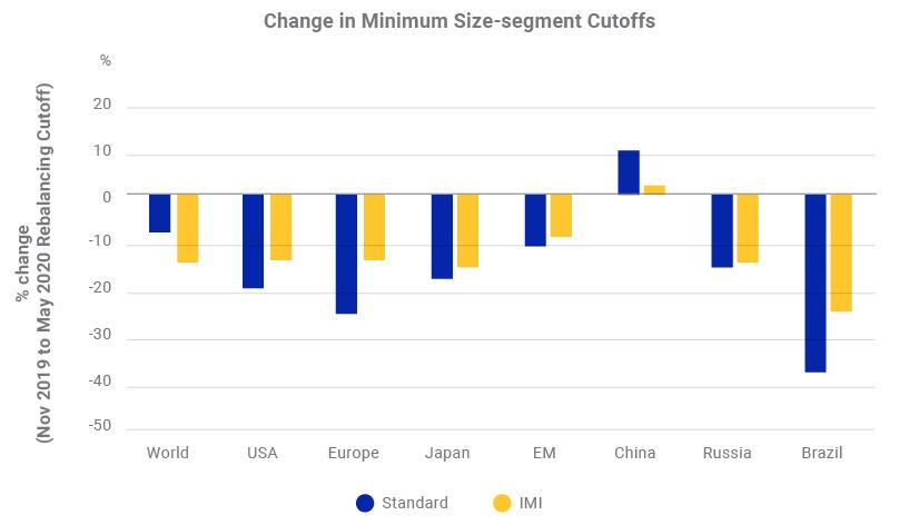
That chart is a reminder that a membership change is not necessarily an error. But failing to represent it correctly creates either survivorship bias or an uninvestable backtest.

Maintain a membership history table rather than a current list of tickers:

universe_id
security_id
effective_start
effective_end
eligible
change_reason
available_at
source_version

For each rebalance date, eligibility requires both:

$$\text{effective start}\le \text{rebalance date}\le \text{effective end}$$

and

$$\text{available at}\le \text{decision time}$$

The first condition models when membership was economically effective. The second models when your research system could know it.

A simple snapshot function makes additions and removals visible:

def eligible_universe_snapshot(
    membership,
    universe_id,
    rebalance_date,
    decision_time,
):
    active_on_date = (
        membership["effective_start"].le(rebalance_date)
        & (
            membership["effective_end"].isna()
            | membership["effective_end"].ge(rebalance_date)
        )
    )

    known_at_decision = (
        membership["available_at"].le(decision_time)
    )

    eligible = (
        membership["universe_id"].eq(universe_id)
        & membership["eligible"]
        & active_on_date
        & known_at_decision
    )

    return set(membership.loc[eligible, "security_id"])


previous_members = eligible_universe_snapshot(
    membership=membership_history,
    universe_id="strategy_universe",
    rebalance_date=previous_rebalance_date,
    decision_time=previous_decision_time,
)

current_members = eligible_universe_snapshot(
    membership=membership_history,
    universe_id="strategy_universe",
    rebalance_date=current_rebalance_date,
    decision_time=current_decision_time,
)

universe_changes = {
    "additions": sorted(current_members - previous_members),
    "removals": sorted(previous_members - current_members),
    "unchanged": sorted(current_members & previous_members),
}

In a production-quality pipeline, add these membership checks:

1. Stable identifier check: use a permanent security_id, not a ticker alone. A ticker or vendor symbol can change after a merger, rebrand, listing migration, or share-class event.
2. Interval validity check: each record has effective_start <= effective_end when an end date exists.
3. Overlap check: a security cannot have contradictory active membership records for the same universe and date.
4. Availability check: no membership revision is used before its available_at timestamp.
5. Change-log check: every addition and removal has a source version and reason code.
6. Expected-panel check: securities outside the point-in-time universe must not be treated as “missing” inputs for that date.
7. Survivorship check: historical snapshots must include assets that later delisted or left the benchmark when they were eligible at the historical decision time.

The identifier issue deserves particular emphasis. A ticker change should not create a fake removal followed by a fake addition. Conversely, a new share class that happens to resemble an old ticker must not be treated as the same economic instrument without reference-data evidence.

---

Build one reusable quality gate

At this point, avoid scattering checks across notebook cells. A compact quality gate can collect issue tables and decide whether a research run may continue.

def make_issues(
    df,
    mask,
    check_name,
    severity,
    evidence_columns,
):
    issues = df.loc[mask, evidence_columns].copy()
    issues["check_name"] = check_name
    issues["severity"] = severity
    return issues


def validate_daily_panel(
    expected_panel,
    canonical_prices,
    return_threshold=0.30,
):
    issues = []

    expected = (
        expected_panel["is_expected_session"]
        & expected_panel["is_eligible"]
    )

    issues.append(
        make_issues(
            expected_panel,
            expected
            & expected_panel["gross_total_return"].isna(),
            check_name="missing_expected_return",
            severity="error",
            evidence_columns=[
                "security_id",
                "trade_date",
                "observation_status",
            ],
        )
    )

    duplicate_key = canonical_prices.duplicated(
        ["security_id", "trade_date"],
        keep=False,
    )

    issues.append(
        make_issues(
            canonical_prices,
            duplicate_key,
            check_name="duplicate_security_date",
            severity="error",
            evidence_columns=[
                "security_id",
                "trade_date",
                "unadjusted_close",
                "source_version",
            ],
        )
    )

    large_return = (
        expected_panel["gross_total_return"].abs()
        > return_threshold
    )

    issues.append(
        make_issues(
            expected_panel,
            large_return,
            check_name="large_return_requires_reconciliation",
            severity="warning",
            evidence_columns=[
                "security_id",
                "trade_date",
                "gross_total_return",
            ],
        )
    )

    return (
        pd.concat(issues, ignore_index=True)
        .sort_values(["severity", "security_id", "trade_date"])
    )

The final gate should stop the run when unresolved errors exist:

quality_issues = validate_daily_panel(
    expected_panel=expected_panel,
    canonical_prices=validated_prices,
)

fatal_issues = quality_issues.loc[
    quality_issues["severity"].eq("error")
]

if not fatal_issues.empty:
    raise RuntimeError(
        "Data quality gate failed. "
        "Review the issue ledger before estimating inputs."
    )

Warnings should not vanish, either. Save them beside the optimizer inputs and backtest outputs. Later, when a performance result looks suspicious, you can inspect precisely which data anomalies were present at each rebalance.

---

Key takeaways

Automated validation is a core part of quantitative portfolio research, not administrative cleanup.

• Define each table’s grain before checking duplicates. For a canonical daily panel, it is usually one row per security and trade date.
• Evaluate missingness against an explicit expectation based on the calendar and point-in-time eligible universe.
• Use schema validation for structure, types, required fields, nullability, and compound keys; use separate business controls for market and portfolio logic.
• Treat extreme returns as investigation triggers. Combine absolute thresholds with rolling, prior-only robust statistics.
• Reconcile raw prices with active corporate actions, and keep adjustment conventions and share bases explicit.
• Use either independently rebuilt total returns or a documented vendor total-return series. Never add distributions to an already total-return-adjusted return.
• Store historical universe membership with effective dates, availability timestamps, reasons, source versions, and stable security identifiers.
• Preserve every issue in a run-level ledger, and prevent the optimizer or backtest from running when fatal data errors remain unresolved.

Next, you will move into return and risk estimation, beginning with how sampling frequency and lookback-window choices affect the means, volatilities, and covariances that feed a portfolio optimizer.