Identifying Training-Serving Skew in Production ML Designs

Hello. In the previous lesson, you separated consistency requirements for features, predictions, and model metadata. That gives us the vocabulary to recognize a particularly common production failure: the model was trained under one input contract but is served under another.

This lesson focuses on identifying training-serving skew in an ML design. By the end, you should be able to inspect a proposed architecture or incident description, distinguish implementation skew from ordinary data drift, and name the evidence needed to prove the diagnosis. This is a useful system-design skill: “we use a feature store” is not, by itself, proof that training and serving are aligned.

---

The prediction contract must be the same

A trained model does not consume a business concept such as “customer risk” or “support-ticket urgency.” It consumes a particular representation of available information: feature names, types, ordering, transformations, default values, and learned preprocessing parameters.

We can describe that representation abstractly as:

$$\mathbf{x}_{\mathrm{train}} = \Phi_{\mathrm{train}}(\text{historical raw data}, t, \text{feature contract})$$

during training, and:

$$\mathbf{x}_{\mathrm{serve}} = \Phi_{\mathrm{serve}}(\text{live request and state}, t, \text{feature contract})$$

during inference.

Training-serving skew exists when these two paths differ in a way that changes what the model actually sees or the population on which it operates. The difference can be caused by an implementation discrepancy, a temporal change in data, or a feedback loop created by the model’s own decisions.

The critical nuance is that the raw inputs do not need to be identical. A ticket classifier trained last month will obviously receive different ticket text today. The contract does need to be compatible:

• the same feature meanings;
• equivalent transformations;
• compatible schemas and types;
• valid time semantics;
• the same handling of missing, malformed, and novel values;
• the correct tokenizer, feature vocabulary, normalization constants, thresholds, or prompt/template package where applicable.

A useful operational test is:

If a logged production request is replayed through the offline pipeline using the same feature and model versions, should it produce the same transformed vector and prediction?

For deterministic models and preprocessing, the answer should be “yes,” apart from explicitly documented nondeterminism such as stochastic sampling. If it does not, the system has an engineering skew until proven otherwise.

{"type":"reading","par_intro":"Read Google for Developers’ *Rules of Machine Learning* for a concise, production-oriented definition of training-serving skew and a diagnostic framework that separates pipeline mismatch from temporal changes and feedback effects.","par_directions":"In the “Training-Serving Skew” section, read <span data-type=\"resource_reading_textrange\" data-resource-subitem-id=\"02ae4e7c\" data-range-start=\"Training-serving skew is a difference between performance during training and performance during serving.\" data-range-end=\"A feedback loop between your model and your algorithm.\">the definition and causes</span>. Then read Rules #29 through #37. In particular, in Rule #31 examine changing lookup tables; in Rule #32 read <span data-type=\"resource_reading_textrange\" data-resource-subitem-id=\"d27b2e3b\" data-range-start=\"Batch processing is different than online processing.\" data-range-end=\"This eliminates a source of training-serving skew.\">the code reuse discussion</span>; and in Rule #36 read <span data-type=\"resource_reading_textrange\" data-resource-subitem-id=\"c59464a6\" data-range-start=\"The position of content dramatically affects how likely the user is to interact with it.\" data-range-end=\"you will be convinced it is more likely to be clicked.\">the ranking feedback example</span>. Finish with Rule #37 and <span data-type=\"resource_reading_textrange\" data-resource-subitem-id=\"38deb3e8\" data-range-start=\"There are several things that can cause skew in the most general sense.\" data-range-end=\"Thus, a discrepancy here probably indicates an engineering error.\">its comparison framework</span>. Focus on what each performance gap can and cannot establish.","learning_duration":"12 minutes","url":"https://developers.google.com/machine-learning/guides/rules-of-ml","title":"Rules of Machine Learning: | Google for Developers","isV2":true,"blockId":"cebfcb12-8437-46f8-a2ee-1e2be67947f2","lessonId":"5b6c4c19-24c9-4b37-9278-c993e4adce39"}

---

Four forms of skew you should recognize

The phrase “skew” is sometimes used too broadly. A better design review distinguishes the following cases, because their evidence and fixes differ.

1. Transformation or schema skew

This is the most direct engineering failure. Training and serving compute a nominally identical feature differently.

Consider a support-ticket urgency model with a feature named open_incidents_7d.

• Offline training computes it from event-time records over the preceding seven complete days.
• The online service calls a counter that actually represents incidents created in the preceding 24 hours.
• Both values are numeric and plausibly correlated with urgency.
• Yet they have different semantics, ranges, and effects on the fitted model.

Other familiar variants include:

• training standardizes a value using saved mean and standard deviation, while serving calculates statistics from the current request batch;
• the batch path treats an absent value as the training median, but online code substitutes zero;
• the model was trained with a fixed categorical vocabulary, while serving hashes unseen categories differently;
• a Python feature pipeline rounds a ratio differently from a separately maintained Java or SQL implementation;
• training uses UTC day boundaries, while the serving path applies a local business timezone;
• an inference service swaps feature order despite retaining the same feature names.

This form is especially dangerous because aggregate dashboards can look healthy. Latency is normal, no infrastructure has failed, and every request has a numeric feature vector. The model simply receives a different problem from the one it learned.

2. Temporal and availability skew

The previous lesson’s point-in-time principle is central here. Historical training examples must be built from information production could have observed at the relevant decision time.

For a labeled example at time $t$, a basic requirement is:

$$t_{\mathrm{feature\ available}} \leq t$$

Violating that condition gives the offline model information from the future. Common causes include backfilled source tables, labels accidentally entering features, and joins against a current dimension table rather than the historical version known at the time.

For example, a malware model may be trained with an IP reputation score that was corrected two days after a file was first seen. If the historical training join uses the corrected score, offline evaluation benefits from information unavailable to the real-time inference service. The online model then underperforms even if the batch and serving code are otherwise identical.

Temporal skew also occurs when the online path uses a legitimate but different freshness contract from training. Suppose the model was trained on a daily customer-profile snapshot but serving reads a feature replica that may be 15 minutes stale. This is not necessarily a defect; it is a design decision. It becomes skew if the training data does not simulate the serving contract, or if the model depends on changes within that staleness window.

3. Population or distribution skew

Features can be computed correctly in both environments while their distributions change between training and serving. This is often called data drift or covariate shift. Google’s broader use of training-serving skew includes this category, but it is important not to misdiagnose it as a code bug.

Examples:

• an energy-price model trained under normal seasonal conditions is served during an unusual supply disruption;
• a new product segment introduces values absent from the historical categorical vocabulary;
• a data-source migration changes the null rate of account fields;
• a fraud model sees a new attack pattern.

The question is whether the population genuinely changed or whether the production feature pipeline changed its meaning. You need feature definitions, provenance, and a replay test to distinguish those possibilities.

{"type":"image","url":"https://docs.cloud.google.com/static/gemini-enterprise-agent-platform/machine-learning/model-monitoring/images/skew_detection_distribution.png","caption":"The Feature distribution comparison shows histograms for the same feature in prediction traffic (top) and training data (bottom), illustrating how a monitoring system can surface a possible training-serving distribution difference.","isV2":true,"blockId":"adfbef1b-3be6-466b-99d8-d26a34e991c8","lessonId":"5b6c4c19-24c9-4b37-9278-c993e4adce39"}

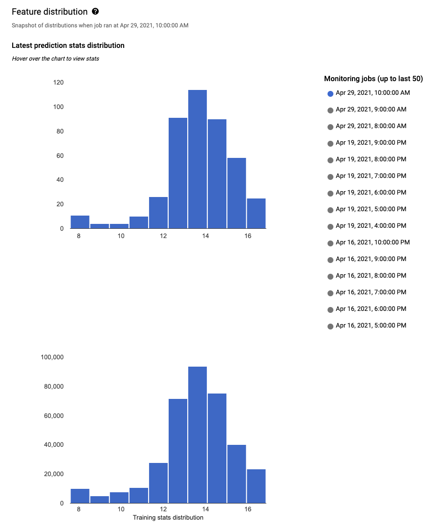
The chart is a useful triage signal, not proof. The two plots have radically different sample counts, so compare normalized bin proportions, quantiles, missing-value rates, and category frequencies rather than raw bar heights. More importantly, similar distributions do not prove feature parity. A serving feature could be shifted, clipped, or incorrectly encoded in a way that preserves a superficially similar histogram.

4. Feedback-loop skew

Some models alter the data from which they are later trained. Ranking, recommendation, spam filtering, fraud intervention, and support-automation systems all have this property.

A ranking model may show an item near the top of a page. Its position affects click probability; clicks are later interpreted as training labels; the next model learns from a population shaped by the previous ranking policy. If the model changes substantially, future logged data no longer represents the distribution that produced the old training set.

This is not solved merely by sharing feature code. The pipeline can be perfectly consistent and still learn a biased view of user preference because it only observes what the system chose to expose. Identifying this category requires asking:

• Which examples are withheld, blocked, ranked down, or never shown?
• Are labels observed for all eligible examples or only selected ones?
• Did a model, threshold, or routing rule change before the performance regression?
• Is position, exposure, or intervention policy represented in the data?

{
  "type": "exercise",
  "id": "51809fa8-d539-4844-be54-b03b22f7690f"
}

---

A production design review: where skew hides

When reviewing a design, trace one prediction backward from the inference endpoint. Do not stop at “the online store serves the same feature names.” For each input, establish its full lineage.

Contract element	Skew-indicating design clue	Evidence to request
Feature definition	Separate SQL and application implementations of the same feature	Versioned definition, code review, golden test cases
Time semantics	Training joins a current table; serving reads live state	Event timestamps, availability timestamps, point-in-time join logic
Preprocessing	Tokenizer, scaler, vocabulary, or imputer is loaded separately from model artifact	Immutable preprocessing artifact digest and deployment manifest
Schema	Features are identified by positional array index or weakly typed JSON	Feature schema, signature validation, request-validation failures
Defaults	Online timeout becomes zero or an empty string without an explicit missingness signal	Missing-value policy and online missingness metrics
Feature freshness	Training uses exact historical snapshots but serving reads an eventually consistent replica	Observed feature-age distribution and fallback policy
Model package	Weight artifact is versioned but tokenizer, threshold, or decision policy is not	A single versioned inference bundle
Label generation	Training labels depend on prior model decisions or selective user exposure	Sampling policy, exposure logs, holdout traffic design

A centralized feature repository can reduce several of these risks, but its presence is not a magic guarantee. A feature store must still provide compatible offline and online definitions, point-in-time-correct historical retrieval, explicit schemas, and meaningful versioning.

{"type":"reading","par_intro":"Read this AWS Machine Learning Lens guidance as a compact checklist for architectural anti-patterns that create feature-level skew, particularly separate transformations, storage formats, and unversioned definitions.","par_directions":"Read the opening “MLREL03-BP02 Verify feature consistency across training and inference” guidance and the “Common anti-patterns” list. Then, in “Implementation guidance,” read from <span data-type=\"resource_reading_textrange\" data-resource-subitem-id=\"706e57c9\" data-range-start=\"Feature consistency between training and inference is critical for\" data-range-end=\"that provides consistent access to the same feature definitions and transformations across both training and inference environments.\">the explanation of the failure mode</span>. Continue through the “Implementation steps,” focusing on the requirement that the offline training path and online inference path use the same feature definitions and transformations, while still using storage appropriate to each workload.","learning_duration":"7 minutes","url":"https://docs.aws.amazon.com/wellarchitected/latest/machine-learning-lens/mlrel03-bp02.html","title":"MLREL03-BP02 Verify feature consistency across training and inference - Machine Learning Lens","isV2":true,"blockId":"4bad9374-92e1-49b8-af28-2c8aa4d5446b","lessonId":"5b6c4c19-24c9-4b37-9278-c993e4adce39"}

---

Diagnosing an apparent quality regression

Suppose a production support-triage model’s offline F1 score is $0.86$, but its delayed live-label F1 score falls to $0.68$. “There is skew” is a reasonable initial hypothesis, but it is not yet a diagnosis.

Use a sequence of increasingly decisive comparisons.

1. Compare training, holdout, future, and live performance

The Google framework is a strong first partitioning of the problem:

Comparison	What a large gap usually suggests
Training versus holdout	Overfitting, evaluation leakage, or an unrepresentative split
Holdout versus chronologically later data	Temporal drift, unstable features, or an incorrect validation scheme
Later offline data versus production replay of the same examples	Pipeline, feature retrieval, preprocessing, or deployment error
Production model score versus replayed offline score for identical inputs	High-confidence implementation skew

The last comparison is particularly powerful. If the same raw production payload, model bundle, and feature values give different scores in offline replay and in production, a change in the external world cannot explain it.

2. Compare feature vectors before comparing aggregate distributions

Take a privacy-safe sample of production requests. For each request, preserve or reconstruct:

• request or event ID;
• prediction timestamp;
• feature-contract version;
• model-bundle version;
• raw or recoverable source references;
• transformed feature vector, or per-feature hashes where raw logging is prohibited;
• missingness indicators and feature ages;
• resulting score and decision.

Recreate the example offline using the declared versions. Compare features one by one, including type and missingness, before looking at model outputs. A single high-impact mismatch can be hidden by a benign overall distribution.

For structured models, a comparison record might look conceptually like this:

Field	Offline reconstruction	Live serving value	Interpretation
open_incidents_7d	19	3	Different window or source
customer_tier	enterprise	enterprise	Matches
last_response_hours	missing	0	Defaulting mismatch
country_code	CZ	127	Encoding mismatch
Model score	0.91	0.54	Explained by input mismatch

For an LLM classifier, equivalent artifacts include the rendered prompt template version, tokenizer version, retrieval configuration, retrieved document IDs, and output schema. The principle remains the same: record enough lineage to reconstruct the actual inference contract without indiscriminately storing sensitive request content.

3. Check system changes before assuming the model decayed

Skew incidents are often introduced by ordinary engineering work:

• a feature source moves from batch to streaming ingestion;
• a timestamp column changes units;
• a service deploy changes a default timeout;
• a new categorical value appears after a product launch;
• a model artifact is promoted without its paired vocabulary or transform package;
• a backfill corrects historical data but the training snapshot reference remains ambiguous;
• an upstream service begins returning partial records.

This is why every prediction should be attributable to an immutable model bundle and feature-contract version, as discussed in the previous lesson. Without that lineage, “the model regressed” becomes a broad forensic exercise rather than a bounded comparison.

{
  "type": "exercise",
  "id": "3593fab9-a90c-42f9-8f88-a0c56e9c4801"
}

---

Preventing skew through shared, testable artifacts

The most reliable prevention is not a promise that two teams will keep their implementations synchronized. It is to reduce the number of independently implemented interpretations.

A production-grade pattern has four components:

1. One versioned feature and schema contract
   Each feature specifies its entity key, type, transformation, time semantics, null behavior, owner, and compatibility policy.

2. Shared or packaged preprocessing
   The fitted vocabulary, normalization constants, bucketing boundaries, tokenizer, and preprocessing logic travel with the model bundle rather than being recreated manually in serving code.

3. Golden parity tests
   Maintain representative raw examples, including nulls, malformed values, rare categories, time-boundary cases, and newly introduced values. Both training and serving paths must produce the expected transformed representation.

4. Production replay and monitoring
   Sample serving requests for replay. Monitor distributions, missingness, feature age, schema violations, unseen-category rate, feature-vector parity failures, and delayed quality metrics.

The TensorFlow Extended example illustrates the general packaging principle: transformations that require full-dataset statistics can be materialized into a transformation graph and reused at training and serving. The important idea is not that every system must use TFX; it is that preprocessing parameters must be immutable, traceable artifacts rather than separately reconstructed operational logic.

{"type":"video","title":"TensorFlow Extended (TFX) Overview and Pre-training Workflow (TF Dev Summit '19)","learning_duration":109,"video_id":"A5wiwT1qFjc","par_intro":"Watch the “Transform” segment of TensorFlow’s *TensorFlow Extended (TFX) Overview and Pre-training Workflow*. It shows a concrete approach to eliminating a common skew source: separate implementations of fitted preprocessing.","par_directions":"In the “Transform” section, watch <span data-type=\"resource_video_timerange\" data-resource-subitem-id=\"fd2264fc\" data-range-start=\"1570\" data-range-end=\"1679\">shared transformations</span>. Focus on why scaling, vocabulary creation, and bucket boundaries require dataset-level statistics, and how packaging those derived constants with the transformation graph lets raw inputs be handled consistently at training and serving.","video_duration":1894,"isV2":true,"blockId":"2937eee8-fb17-48b4-91ae-2e80c906e32c","lessonId":"5b6c4c19-24c9-4b37-9278-c993e4adce39"}

{
  "type": "exercise",
  "id": "bbc09588-70bc-4216-a8dd-a427cedc8873"
}

---

A concise senior-level diagnosis statement

In an interview or design review, a strong answer does more than name “feature drift.” It specifies the violated contract and the test that would establish it. For example:

“I would suspect training-serving skew because training computes the incident-count feature with an event-time seven-day window, while online inference reads a near-real-time aggregate whose window and staleness are not specified. I would first replay sampled production requests through the offline feature pipeline using the exact deployed model bundle. If feature values or scores differ for the same request, that is an implementation skew. If parity holds but feature distributions and performance changed after the product launch, I would treat it as population drift or a feedback effect rather than a transformation bug.”

That answer communicates the distinction between:

• a semantic mismatch in a feature pipeline;
• a temporal mismatch caused by unavailable future information;
• a real population shift;
• a policy-induced feedback loop.

---

Key takeaways

Training-serving skew is a mismatch between the prediction conditions a model learned from and the conditions under which it is deployed. It can arise from separate feature transformations, incompatible schemas or defaults, incorrect historical time joins, genuine population changes, or model-induced feedback loops.

To identify it reliably:

• treat features, preprocessing, and model-associated assets as one versioned prediction contract;
• distinguish drift in the world from a mismatch in implementation;
• replay identical production examples through the offline path;
• compare individual feature vectors before relying on aggregate distribution charts;
• log versioned lineage, missingness, freshness, and relevant exposure information;
• use shared artifacts and parity tests to prevent two pipelines from silently diverging.

Next, you will turn these diagnostic ideas into operational commitments by defining service-level indicators and objectives for an ML-powered service.