Japan's Liquidity Trap: An Empirical Assessment

Hello! Welcome to the fifth and final lesson of our module on Japan's deflationary era.

In our last lesson, we evaluated the effectiveness of the Bank of Japan's major policy responses, ZIRP and QE. We concluded that even the most aggressive "shock and awe" policies under Abenomics failed to generate sustained, demand-driven inflation, suggesting that something was blocking the monetary transmission mechanism. The most common explanation for this phenomenon is the liquidity trap.

Introduction

Today, we will put that very explanation under the microscope. Our goal is to address the learning outcome: Critically assess the argument that Japan was in a liquidity trap, using the empirical criteria developed earlier to analyze relevant data.

This is a crucial lesson that brings together several threads from our course. We will move beyond accepting the liquidity trap as a given and instead treat it as a testable hypothesis.

• Estimated time to complete: 60 minutes.
• Recap: In our very first module (Lesson 1.5), we established the empirical criteria for identifying a liquidity trap within an IS-LM framework:
  1. Nominal short-term interest rates are at or near the Zero Lower Bound (ZLB).
  2. The interest elasticity of money demand is extremely high (approaching infinite), implying a horizontal LM curve. This is the condition that renders conventional monetary policy ineffective.

We will use these criteria to structure our critical assessment.

---

1. The Conventional View: Japan as the Textbook Liquidity Trap

The narrative that Japan fell into a liquidity trap is pervasive in economics textbooks and commentary. The prima facie evidence is compelling and aligns perfectly with our first criterion.

Video & Visual Evidence (5 minutes):

First, watch this brief clip which explicitly names Japan as a prime example of a liquidity trap.

Now, let's look at the data. The following charts clearly illustrate the conditions that gave rise to this view.

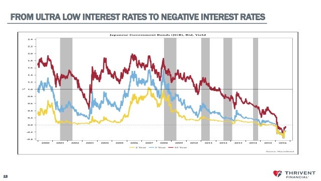
This graph powerfully illustrates that Criterion 1 was met. From the late 1990s, short-term and even medium-term (2- and 5-year) Japanese Government Bond (JGB) yields collapsed towards zero, eventually turning negative.

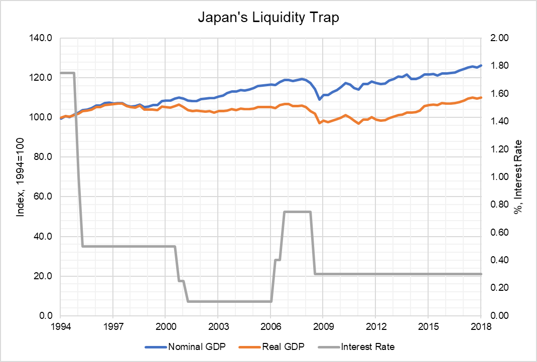
This chart shows the result. Despite interest rates (grey line) being pinned near zero for two decades, real GDP growth (orange line) remained stubbornly low. This is the classic image of "pushing on a string."

The conventional argument, famously advanced by Paul Krugman, is that once rates hit zero, the Bank of Japan's open market operations (swapping central bank reserves for government bonds) became useless. At the ZLB, short-term bonds and money are near-perfect substitutes, so swapping one for the other has no effect. People and firms, pessimistic about the future and expecting deflation, simply hoard the extra cash rather than spending or investing it. This implies a perfectly elastic demand for money—a horizontal LM curve.

This narrative is simple, powerful, and fits the surface-level facts. But is it empirically robust?

---

2. Counter-Argument I: A Vertical IS Curve, Not a Horizontal LM Curve

The first major empirical challenge to the standard liquidity trap story comes from a different interpretation of the IS-LM model. What if the problem wasn't with the LM curve (monetary policy) but with the IS curve (the real economy)?

Economists Naoyuki Yoshino and Farhad Taghizadeh-Hesary argue precisely this. Their hypothesis is that Japan's stagnation was caused by a vertical IS curve, meaning that investment and consumption had become completely insensitive to changes in the real interest rate.

Reading & Analysis (20 minutes):

Please read the following sections from their 2015 paper. Given your background, you'll find their use of a Seemingly Unrelated Regressions (SUR) model to estimate the IS-LM system quite accessible.

Japan's Lost Decade: Lessons for Other Economies (Abstract and Introduction to the Liquidity Trap Argument; Ineffective Monetary Policy and Vertical IS Curve; Empirical Analysis of IS-LM Model; Empirical Results and Rejection of Liquidity Trap)

As you read, focus on these key questions:

• How do the authors frame their argument against Krugman's liquidity trap hypothesis in the introduction?
• Examine the empirical results in Table 5.
  • In the IS equation, what does the coefficient and statistical significance of the real interest rate (i-p) tell you about the slope of the IS curve?
  • In the LM equation, what do the coefficients on real GDP (y) and the nominal interest rate (i) tell you about the slope of the LM curve? Is it horizontal?

My Explanation:

The results of this study are a direct contradiction of the textbook liquidity trap story.

1. The IS Curve is Vertical: The regression for the IS equation finds that the coefficient on the real interest rate is statistically insignificant (p-value = 0.60). This is strong evidence that changes in the real interest rate had no discernible effect on real GDP. Investment was simply not responding to lower borrowing costs.
2. The LM Curve is Upward-Sloping: The regression for the LM equation finds statistically significant coefficients for both real income (positive) and the interest rate (negative) on money demand. This implies a standard, upward-sloping LM curve, not the horizontal curve required for a liquidity trap.

This evidence suggests that our second criterion for a liquidity trap was not met. The problem wasn't that monetary policy was powerless, but rather that the real economy was unresponsive. The "string" wasn't being pushed; it was connected to an object that was bolted to the floor. This points toward deep structural issues, which we'll begin to explore in the next lesson.

---

3. Counter-Argument II: Was Monetary Policy Really Ineffective?

A second, more methodologically advanced challenge comes from a 2020 Bank for International Settlements (BIS) working paper. Instead of estimating static IS-LM curves, the authors use a Bayesian Structural Vector Autoregression (SVAR) model to analyze the dynamic effects of monetary policy.

Their approach is clever: they compare the impact of an expansionary monetary policy shock during "normal times" (pre-1996) with its impact during "ELB (Effective Lower Bound) times" (1996 onwards). If a liquidity trap exists, the impact of monetary policy shocks during ELB times should be significantly weaker or non-existent.

Reading & Analysis (20 minutes):

These sections from the paper outline the methodology and the striking results for Japan. Your econometrics background will be very helpful here in appreciating the impulse-response analysis.

Does the liquidity trap exist? (Defining ELB Times and Data for Japan; Monetary Policy Effectiveness at ELB; Dynamic Effects of Monetary Policy Shocks in Japan; Conclusion: Liquidity Trap as a Theoretical Concept)

As you read, focus on:

• The authors' definition of "ELB times" for Japan.
• The core logic of their argument: that unconventional policies can still work through channels other than short-term rates (e.g., credit, asset prices, expectations).
• The key results in Figure 10(a). Compare the impulse response functions (IRFs) for industrial production (ipt) and prices (pt) during normal times (red) versus ELB times (blue). Is the response weaker during the ELB period?
• The paper's final conclusion in Section V.

My Explanation:

The findings of this paper are remarkable and turn the conventional liquidity trap narrative on its head.

Does the liquidity trap exist? (Figures and Tables for Japan)
This figure shows the Impulse Response Functions (IRFs) for Japan. A one-time expansionary monetary policy shock is simulated in both the pre-1996 "normal" period (red) and the post-1996 "ELB" period (blue).

Look closely at the top two panels of Figure 10(a). In response to an expansionary monetary policy shock:

• Output (ipt): The response during ELB times (blue line) is both faster and four times larger in magnitude than the response during normal times (red line).
• Prices (pt): The response is also significantly stronger and faster during the ELB period.

This is the exact opposite of what a liquidity trap would predict. The authors argue that while conventional policy was constrained, unconventional policies (QE, forward guidance) working through credit and asset price channels were not only effective but more effective, likely because the economy was more financially constrained during the crisis period.

Their conclusion is stark: the "Hicks-type liquidity trap" has been "more of a theoretical concept than an empirical reality."

---

Conclusion

Today we critically assessed the claim that Japan was in a liquidity trap. While the narrative is compelling and fits the surface-level data of zero interest rates and low growth, it does not stand up well to rigorous empirical testing.

Key Takeaways:

• Criterion 1 (ZLB) was met: There is no doubt that Japan's policy rates were at the Zero Lower Bound for decades.
• Criterion 2 (Horizontal LM / Ineffective Monetary Policy) is not supported by the data:
  • IS-LM estimations suggest the problem was a vertical IS curve (unresponsive investment), not a horizontal LM curve.
  • SVAR analysis shows that unconventional monetary policy was not only effective at the ELB, but potentially more effective than during normal times.
• The diagnosis matters: Misdiagnosing the problem as a liquidity trap (an LM curve issue) led to a focus on ever-more extreme monetary policy. The evidence suggests the root cause was structural (an IS curve issue), which monetary policy alone could not fix.

Next Lesson Preview:

Our conclusion that the problem was structural, not a simple liquidity trap, provides the perfect bridge to our next module. If a broken monetary transmission mechanism wasn't the primary culprit, what was? In our next lesson, we will begin to answer this by investigating the first major confounding variable: the role of Japan's 1990s banking crisis and its long-term effects on credit creation and investment ('credit crunch').