Gradient Descent Updates and the Impact of Learning Rate and Feature Scale

Good to see you again. Last lesson established the key quantity that drives training: for average half-squared error,

$$J(\mathbf{w})=\frac{1}{2n}{\Vert \mathbf{Xw}-\mathbf{y}\Vert }_2^2$$

the gradient is

$${\nabla }_{\mathbf{w}}J=\frac{1}{n}{\mathbf{X}}^{\top }\left(\mathbf{Xw}-\mathbf{y}\right)$$

It is a vector of feature–residual alignments: its sign tells us which way to change each coefficient locally, and its magnitude tells us how strongly the loss responds.

This lesson turns that local information into an optimization algorithm. You will perform gradient-descent updates, see precisely why the learning rate can make training slow, stable, oscillatory, or divergent, and connect feature scaling to the geometry of the loss surface.

---

From a gradient to a parameter update

At the current parameter vector ${\mathbf{w}}^{(t)}$, the first-order approximation from the previous lesson is

$$J({\mathbf{w}}^{(t)}+\Delta \mathbf{w})\approx J({\mathbf{w}}^{(t)})+\nabla J({\mathbf{w}}^{(t)}{)}^{\top }\Delta \mathbf{w}$$

The gradient points in the direction of greatest local increase in loss. To reduce loss, choose a small displacement in the opposite direction:

$$\Delta \mathbf{w}=-\eta \nabla J({\mathbf{w}}^{(t)})$$

where $\eta >0$ is the learning rate, also called the step size. Substitution gives the gradient-descent update:

$$\boxed{{\mathbf{w}}^{(t+1)}={\mathbf{w}}^{(t)}-\eta \nabla J({\mathbf{w}}^{(t)})}$$

For squared-error linear regression, insert the gradient derived previously:

$$\boxed{{\mathbf{w}}^{(t+1)}={\mathbf{w}}^{(t)}-\frac{\eta }{n}{\mathbf{X}}^{\top }\left(\mathbf{X}{\mathbf{w}}^{(t)}-\mathbf{y}\right)}$$

All coordinates of $\mathbf{w}$ are updated simultaneously, using the gradient evaluated at the old parameter vector. Updating one coefficient and then using that new value while computing the next coefficient creates a different algorithm.

The central loop is conceptually simple:

1. Compute predictions and residuals using the current parameters.
2. Compute the gradient of the loss.
3. Multiply the gradient by the learning rate.
4. Subtract that scaled gradient from the parameters.
5. Repeat until the loss or parameter updates have stabilized, or a stopping budget is reached.

The procedure applies far beyond linear regression. Only the loss and its gradient change for logistic regression, neural networks, boosted models, and many other estimators.

---

One complete batch-gradient update

Continue with the two-observation regression example from the prior lesson:

$$\mathbf{X}=\left[\begin{array}{cc}1& 2\\ 1& 4\end{array}\right],\mathbf{y}=\left[\begin{array}{c}5\\ 8\end{array}\right],{\mathbf{w}}^{(0)}=\left[\begin{array}{c}1\\ 1\end{array}\right]$$

We already found

$$\nabla J({\mathbf{w}}^{(0)})=\left[\begin{array}{c}-2.5\\ -8\end{array}\right]$$

Choose a learning rate of

$$\eta =0.1$$

The update is

$${\mathbf{w}}^{(1)}=\left[\begin{array}{c}1\\ 1\end{array}\right]-0.1\left[\begin{array}{c}-2.5\\ -8\end{array}\right]$$ $${\mathbf{w}}^{(1)}=\left[\begin{array}{c}1.25\\ 1.8\end{array}\right]$$

Both parameters increase because both gradient components were negative. That is consistent with the initial model underpredicting both target values.

Check whether the loss has improved. The new predictions are

$$\mathbf{X}{\mathbf{w}}^{(1)}=\left[\begin{array}{c}4.85\\ 8.45\end{array}\right]$$

so the residuals are

$${\mathbf{r}}^{(1)}=\left[\begin{array}{c}-0.15\\ 0.45\end{array}\right]$$

The initial loss was $3.25$. The updated loss is

$$J({\mathbf{w}}^{(1)})=\frac{1}{4}\left((-0.15{)}^2+(0.45{)}^2\right)=0.05625$$

One update has reduced the loss sharply. It has not reached zero because the model has two parameters and only moved once from an arbitrary initial setting; further updates would refine it.

A useful operational interpretation is that the learning rate converts the gradient from a direction-and-sensitivity signal into a concrete parameter change. The gradient alone says, “increase both entries.” The learning rate decides whether that increase is cautious, productive, or disastrous.

---

Learning rate: why too small and too large both fail

The learning rate is a hyperparameter: it is chosen by the training process rather than inferred directly as a model coefficient. A single global learning rate must work across all parameter directions, which is why the geometry of the loss matters.

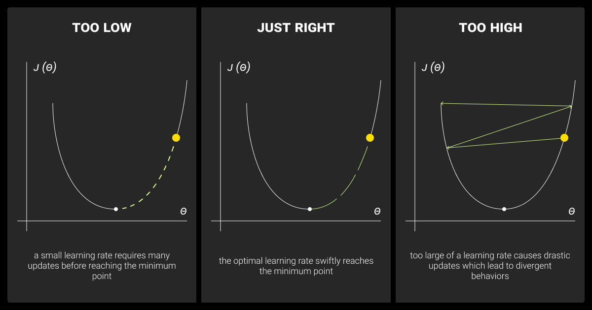
To see the logic exactly, consider a one-parameter quadratic loss centered at its optimum $w^{\star }$:

$$J(w)=\frac{1}{2}\lambda (w-w^{\star }{)}^2$$

Here $\lambda >0$ measures the curvature: a large $\lambda$ means a narrow, steep bowl. Its derivative is

$$\frac{dJ}{dw}=\lambda (w-w^{\star })$$

Gradient descent gives

$$w^{(t+1)}=w^{(t)}-\eta \lambda \left(w^{(t)}-w^{\star }\right)$$

Define the error from the optimum as

$$e^{(t)}=w^{(t)}-w^{\star }$$

Then the update reduces to

$$e^{(t+1)}=\left(1-\eta \lambda \right)e^{(t)}$$

The multiplier $1-\eta \lambda$ determines convergence.

Condition	Behavior
$0<\eta \lambda <1$	Moves toward the minimum without crossing it.
$1<\eta \lambda <2$	Crosses the minimum on each iteration, but oscillations shrink.
$\eta \lambda =2$	Oscillates indefinitely at constant distance from the minimum.
$\eta \lambda >2$	Oscillations grow: gradient descent diverges.
$\eta \lambda \approx 0$	Stable but painfully slow progress.

Thus, for this quadratic, stable convergence requires

$$0<\eta <\frac{2}{\lambda }$$

The important point is not that you will calculate this bound for every model. In realistic optimization, the curvature is multidimensional, may vary across the parameter space, and may be estimated noisily from mini-batches. The point is that a learning rate is only meaningful relative to curvature.

For least-squares linear regression, that curvature is governed by

$$\mathbf{H}=\frac{1}{n}{\mathbf{X}}^{\top }\mathbf{X}$$

the Hessian of the loss. Its largest eigenvalue corresponds to the steepest curvature direction. A fixed learning rate that is safe in that direction can still produce frustratingly slow movement along a much flatter direction. Feature scaling is one of the main ways to reduce this mismatch.

---

Why feature scale changes optimization geometry

Recall that one component of the squared-error gradient is

$$\frac{\partial J}{\partial w_j}=\frac{1}{n}\sum _{i=1}^n{r}_i{x}_{ij}$$

If feature $x_j$ is measured in thousands while another feature is an integer count from $0$ to $5$, their raw gradient components tend to have very different numerical scales. But the deeper issue is not merely “large gradients.” Rescaling a feature also changes the parameter coordinate system and reshapes the loss surface.

Suppose a house-price model uses:

• floor area, perhaps spanning $300$ to $2000$ square feet;
• bedroom count, perhaps spanning $0$ to $5$.

A useful coefficient for floor area will typically be numerically much smaller than a useful coefficient for bedroom count, because it is multiplied by much larger feature values. The same predictions can be represented either way, but gradient descent has to navigate the resulting loss surface.

Contour lines connect parameter settings with equal loss. In the upper plot, a small change in one parameter has a much larger prediction effect than an equally sized change in the other. The loss surface is therefore a long, narrow valley.

Gradient descent always takes the local steepest direction. In a narrow valley, that direction points substantially across the valley rather than directly along it toward the minimum. The algorithm repeatedly crosses from one side to the other while making only modest progress down the valley. Reducing the learning rate prevents violent oscillation, but then progress along the shallow direction becomes slow.

Scaling features to broadly comparable ranges makes the contours more nearly circular. This improves the conditioning of the optimization problem: curvature varies less dramatically across directions, so one learning rate works more effectively for all coefficients.

---

Standardization changes coordinates, not the underlying model

A common transformation is standardization:

$$z_j=\frac{x_j-{\mu }_j}{s_j}$$

where ${\mu }_j$ is the feature mean in the training data and $s_j$ is its standard deviation. After standardization, each continuous feature has approximately mean $0$ and variance $1$ on the data used to fit the scaler.

For a linear model, standardization does not reduce what the model can represent. It changes the numerical parameterization.

If the original model is

$$\hat{y}=b+\sum _{j=1}^p{w}_j{x}_j$$

and $x_j=s_j{z}_j+{\mu }_j$, it can be written equivalently as

$$\hat{y}=b^{\prime }+\sum _{j=1}^p{w}_j^{\prime }{z}_j$$

where

$$w_j^{\prime }=s_j{w}_j$$

and

$$b^{\prime }=b+\sum _{j=1}^p{w}_j{\mu }_j$$

So scaling affects the numerical values of coefficients, the gradients, and the shape of the optimization landscape, while leaving the set of possible predictions unchanged.

In practice:

• Standardize continuous features when using gradient-based linear models, logistic regression, support-vector methods, neural networks, PCA, or distance-based methods.
• Do not standardize the intercept column of ones.
• Treat binary indicator variables deliberately. Scaling them is sometimes technically acceptable, but it can reduce coefficient interpretability and is often unnecessary.
• Fit the scaling parameters only on training data, then apply those same stored transformations to validation, test, and production data. Re-estimating them separately on test data changes the model’s input coordinate system and leaks distributional information.

---

A compact notebook check

The following code reproduces batch gradient descent for the previous two-observation example. Run it with several learning rates and inspect both the loss history and the parameter values.

import numpy as np

X = np.array([
    [1.0, 2.0],
    [1.0, 4.0],
])

y = np.array([5.0, 8.0])

def loss(w, X, y):
    residuals = X @ w - y
    return 0.5 * np.mean(residuals ** 2)

def gradient(w, X, y):
    residuals = X @ w - y
    return X.T @ residuals / len(y)

def batch_gradient_descent(X, y, eta, n_steps, w0):
    w = w0.astype(float).copy()
    history = [loss(w, X, y)]

    for _ in range(n_steps):
        w = w - eta * gradient(w, X, y)
        history.append(loss(w, X, y))

    return w, np.array(history)

for eta in [0.01, 0.1, 0.2]:
    final_w, history = batch_gradient_descent(
        X=X,
        y=y,
        eta=eta,
        n_steps=20,
        w0=np.array([1.0, 1.0]),
    )

    print(f"\neta = {eta}")
    print("final parameters:", final_w)
    print("first five losses:", history[:5])
    print("final loss:", history[-1])

Interpret the results as an optimization diagnostic rather than as a recipe for universal learning rates:

• With $\eta =0.01$, the loss should fall cautiously but may require many iterations.
• With $\eta =0.1$, this small example makes rapid early progress.
• With $\eta =0.2$, the update is too aggressive for this particular loss geometry and can increase the loss rather than reduce it.

For a full-batch quadratic problem such as this, a repeatedly rising loss is a strong warning that the learning rate is too high. With mini-batch gradient descent, individual batch losses are noisy, so practitioners inspect trends over an epoch or a smoothed moving average rather than demanding a decrease after every update.

---

Key takeaways

Gradient descent updates a parameter vector by subtracting a learning-rate-scaled gradient:

$${\mathbf{w}}^{(t+1)}={\mathbf{w}}^{(t)}-\eta \nabla J({\mathbf{w}}^{(t)})$$

The negative gradient gives the local direction of decreasing loss; the learning rate determines the size of the step. Too small a rate produces stable but slow training. Too large a rate overshoots the minimum, causing oscillation or divergence.

Feature scale matters because it affects the curvature and conditioning of the loss surface. Vastly different feature ranges create elongated contours, forcing gradient descent to zigzag and making one shared learning rate difficult to choose. Standardization commonly makes optimization substantially more efficient, provided that scaling parameters are learned from training data and reused everywhere else.

Next, this module shifts from optimization to the geometry of data itself: you will interpret the eigenvectors and eigenvalues of a covariance matrix as principal directions and magnitudes of variation—the mathematical basis for PCA.