Linear Model Predictions with Dot Products and Matrix Multiplication

Welcome. This course builds a working mathematical backbone for conventional machine learning: enough to inspect a proposed model, reason about its behavior, and communicate precisely with engineers. This first module focuses on the compact linear-algebra notation behind many models and the optimization methods used to fit them.

In this lesson, you will move from the familiar scalar equation of a linear model to two equivalent representations:

1. a dot product for one prediction;
2. a matrix-vector product for predictions across an entire dataset.

The notation is compact, but it is not merely shorthand. It makes clear what a model consumes, what its parameters are, and which dimensions must agree before a pipeline can produce valid predictions.

---

One observation: a prediction is a weighted sum

Suppose a model estimates the weekly number of support tickets for a customer account from two features:

• $x_1$: active users, measured in thousands;
• $x_2$: whether a campaign is running, encoded as $0$ or $1$.

A linear prediction rule might be

$$\hat{y}={\beta }_0+{\beta }_1{x}_1+{\beta }_2{x}_2$$

Here:

• $\hat{y}$ is the model’s prediction;
• ${\beta }_0$ is the intercept, the baseline prediction;
• ${\beta }_1$ and ${\beta }_2$ are coefficients or weights;
• each feature contributes its observed value multiplied by its coefficient.

For example, let

$${\beta }_0=20,{\beta }_1=3,{\beta }_2=8$$

For an account with $4$ thousand active users and an active campaign:

$$\hat{y}=20+3(4)+8(1)=40$$

The interpretation is conditional on the other features being held fixed. In this model, one additional thousand active users changes the predicted ticket count by $3$; enabling the campaign changes it by $8$.

A linear model is therefore linear in its parameters: it combines feature values through weighted addition. The features themselves can still be engineered transformations. For instance, including a feature such as $x_1^2$ allows curved behavior with respect to the original variable while retaining a model that is linear in its coefficients.

Folding the intercept into the feature vector

The intercept is handled neatly by defining a constant feature $x_0=1$. For one observation, write the augmented feature vector and coefficient vector as

$$\tilde{\mathbf{x}}=\left[\begin{array}{c}1\\ x_1\\ x_2\end{array}\right],\mathbf{\beta }=\left[\begin{array}{c}{\beta }_0\\ {\beta }_1\\ {\beta }_2\end{array}\right]$$

The prediction becomes a dot product:

$$\hat{y}={\tilde{\mathbf{x}}}^{\top }\mathbf{\beta }=\sum _{j=0}^p{x}_j{\beta }_j$$

where $p$ is the number of non-intercept features.

For the support-ticket example,

$$\tilde{\mathbf{x}}=\left[\begin{array}{c}1\\ 4\\ 1\end{array}\right],\mathbf{\beta }=\left[\begin{array}{c}20\\ 3\\ 8\end{array}\right]$$

and hence

$${\tilde{\mathbf{x}}}^{\top }\mathbf{\beta }=1(20)+4(3)+1(8)=40$$

The dot product is the fundamental unit of a linear-model prediction: match each feature with its corresponding weight, multiply, and add.

This has an important operational consequence. The order of columns is part of the model contract. If the feature vector is supplied as $[1,\text{campaign},\text{active users}]$ while the coefficient vector expects $[1,\text{active users},\text{campaign}]$, the dimensions still match and the computation succeeds, but the prediction is semantically wrong. Schema enforcement and feature definitions matter as much as successful matrix operations.

---

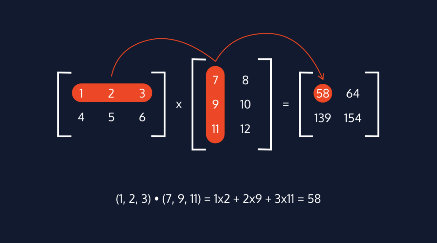
The highlighted row and column in the image below show precisely the calculation for one entry of a matrix product: a row from the left matrix is paired with a column from the right matrix.

---

From one prediction to a whole batch

A model is ordinarily evaluated or deployed over many observations. Rather than write one dot product per account, we stack observations into a design matrix.

Suppose there are $n$ observations and $p$ features, excluding the intercept. Each row is one observation; each non-intercept column is one feature:

$$\mathbf{X}=\left[\begin{array}{ccccc}1& x_{11}& x_{12}& \cdots & x_{1p}\\ 1& x_{21}& x_{22}& \cdots & x_{2p}\\ ⋮& ⋮& ⋮& \ddots & ⋮\\ 1& x_{n1}& x_{n2}& \cdots & x_{np}\end{array}\right]$$

Its shape is

$$\mathbf{X}\in {\mathbb{R}}^{n\times (p+1)}$$

The parameter vector has one coefficient for each column:

$$\mathbf{\beta }=\left[\begin{array}{c}{\beta }_0\\ {\beta }_1\\ ⋮\\ {\beta }_p\end{array}\right]\in {\mathbb{R}}^{(p+1)\times 1}$$

The predicted values for every observation are then

$$\hat{\mathbf{y}}=\mathbf{X}\mathbf{\beta }$$

The shapes explain why this is valid:

$$(n\times (p+1))((p+1)\times 1)=n\times 1$$

The output contains exactly one prediction for each observation.

Object	Meaning	Shape
$\mathbf{X}$	Design matrix: rows are observations, columns are features	$n\times (p+1)$
$\mathbf{\beta }$	Intercept and feature coefficients	$(p+1)\times 1$
$\hat{\mathbf{y}}$	Batch of model predictions	$n\times 1$

The inner dimensions, both $p+1$, must match. The outer dimensions determine the output shape. This is the most reliable mental check for matrix multiplication.

---

---

Working through a batch prediction

Return to the ticket model, and consider two accounts:

Account	Active users, thousands	Campaign active
A	4	1
B	7	0

Including the intercept column, the design matrix is

$$\mathbf{X}=\left[\begin{array}{ccc}1& 4& 1\\ 1& 7& 0\end{array}\right]$$

and the parameter vector is

$$\mathbf{\beta }=\left[\begin{array}{c}20\\ 3\\ 8\end{array}\right]$$

Therefore,

$$\hat{\mathbf{y}}=\mathbf{X}\mathbf{\beta }=\left[\begin{array}{ccc}1& 4& 1\\ 1& 7& 0\end{array}\right]\left[\begin{array}{c}20\\ 3\\ 8\end{array}\right]=\left[\begin{array}{c}1(20)+4(3)+1(8)\\ 1(20)+7(3)+0(8)\end{array}\right]=\left[\begin{array}{c}40\\ 41\end{array}\right]$$

Nothing mysterious happens in the batch operation. The first row produces Account A’s prediction, and the second row produces Account B’s prediction. Matrix multiplication simply performs the same dot-product rule once per row.

In NumPy, this is expressed with the matrix-multiplication operator:

import numpy as np

X = np.array([
    [1.0, 4.0, 1.0],
    [1.0, 7.0, 0.0]
])

beta = np.array([20.0, 3.0, 8.0])

y_hat = X @ beta
# array([40., 41.])

For arrays, @ communicates matrix multiplication directly. In contrast, X * beta performs elementwise multiplication through broadcasting; it produces a matrix of separate products rather than the vector of summed predictions. The final summation across each row is essential.

NumPy commonly represents beta above as a one-dimensional array of shape $(3,)$, and correspondingly returns y_hat with shape $(2,)$. Mathematically, it is useful to retain the column-vector convention because it makes every multiplication and dimension explicit.

---

Predictions, observed targets, and errors

It is worth separating three related expressions that are often compressed into one notation.

A fitted model makes deterministic predictions, given a feature matrix and fitted coefficient vector:

$$\hat{\mathbf{y}}=\mathbf{X}\hat{\mathbf{\beta }}$$

The observed targets are the actual ticket counts, prices, durations, or other measured outcomes:

$$\mathbf{y}=\left[\begin{array}{c}{y}_1\\ ⋮\\ y_n\end{array}\right]$$

The difference between them is the residual vector:

$$\mathbf{r}=\mathbf{y}-\hat{\mathbf{y}}$$

In a statistical model, one commonly writes

$$\mathbf{y}=\mathbf{X}\mathbf{\beta }+\mathbf{ϵ}$$

This says that observed outcomes comprise a systematic linear component plus an error term. At this stage, treat it as a modeling statement, not as an assertion that the model predicts errors. For prediction, the central object is $\hat{\mathbf{y}}=\mathbf{X}\hat{\mathbf{\beta }}$. Later lessons will address how coefficients are fitted by minimizing losses based on residuals.

The same core computation also appears in classification. A linear classifier first produces a score

$$s_i={\tilde{\mathbf{x}}}_i^{\top }\mathbf{\beta }$$

Logistic regression subsequently transforms that score into a probability. The interpretation of the output changes, but the feature–weight dot product remains the computational backbone.

---

A compact review checklist

When reading a linear-model proposal, notebook, or model-serving specification, verify these points:

1. Prediction unit: What does one row represent: a customer, transaction, device-day, or another unit?
2. Feature definition: Which columns appear in $\mathbf{X}$, in what order, with what units and encodings?
3. Intercept convention: Is a column of ones included explicitly, or is an intercept stored separately by the modeling library?
4. Parameter alignment: Does every feature column have exactly one corresponding coefficient?
5. Shape compatibility: If $\mathbf{X}$ is $n\times (p+1)$, is the parameter vector $(p+1)\times 1$?
6. Output meaning: Is $\mathbf{X}\mathbf{\beta }$ a regression prediction, a classifier score, or an intermediate quantity?

These checks catch both obvious matrix-shape errors and more dangerous semantic errors, such as swapped feature columns or inconsistent feature transformations between training and production.

---

A linear-model prediction is a weighted sum. For one observation, it is a dot product:

$${\hat{y}}_i={\tilde{\mathbf{x}}}_i^{\top }\mathbf{\beta }$$

For a dataset, stacking observations as rows gives the equivalent batch computation:

$$\hat{\mathbf{y}}=\mathbf{X}\mathbf{\beta }$$

The column of ones incorporates the intercept, and the shape rule ensures the operation is valid. Most importantly, the mathematical alignment between feature columns and coefficients is also a data-contract requirement in a real ML system.

Next, we will use this notation to compute gradients of scalar loss functions with respect to vector-valued model parameters—the step that turns a prediction rule into a trainable model.