Mastering NumPy Array Shapes, Axes, Indexing, and Broadcasting

Welcome back. In the previous lesson, you used NumPy’s vectorized operations to express computations over entire arrays rather than writing Python loops. That style becomes reliable only when you can reason about an array’s shape: which dimension represents examples, features, channels, or coordinates, and which dimensions an operation expects.

This lesson develops that skill. You will inspect and reshape arrays, reduce data along the right axis, select subsets with indexing, and use broadcasting deliberately rather than treating a dimension error as something to “reshape until it works.” These are everyday concerns in ML preprocessing, training, and inference code.

---

Shape is an interface contract

A NumPy array’s shape describes its extent along each axis. For a two-dimensional array, the conventional interpretation is:

import numpy as np

X = np.array([
    [210, 4.8, 1],
    [175, 3.2, 0],
    [320, 4.1, 1],
    [145, 2.9, 0],
])

print(X.shape)  # (4, 3)
print(X.ndim)   # 2
print(X.size)   # 12

Here, a useful ML interpretation is:

• axis 0: 4 observations, often called the batch or sample axis;
• axis 1: 3 features per observation.

The shape (4, 3) is more than a storage detail. It is a contract: code that expects one row per example and three input features can consume this array correctly. If a preprocessing operation accidentally produces (3, 4), the same twelve values exist, but their meaning has changed.

A helpful rule is:

Read a shape from left to right as the sizes of successive indices.

For X.shape == (4, 3), valid element coordinates have the form X[row, column], where row ranges from 0 to 3, and column ranges from 0 to 2.

For higher-dimensional data, attach a semantic label to each position in the shape rather than trying to visualize all dimensions. For example, image batches often have a shape such as (batch, height, width, channels). A tensor of shape (32, 224, 224, 3) can therefore mean 32 color images, each 224 by 224 pixels with three RGB values per pixel. Different libraries can adopt different dimension conventions, so inspect the documented model-input contract rather than assuming one.

Use .shape constantly while developing:

def inspect_array(name, array):
    print(
        f"{name}: shape={array.shape}, "
        f"ndim={array.ndim}, dtype={array.dtype}"
    )

inspect_array("X", X)
# X: shape=(4, 3), ndim=2, dtype=int64

The exact integer type may differ across operating systems; the important properties here are shape and dimensionality.

Read the relevant parts of NumPy’s official beginner guide now. It establishes the vocabulary used throughout the rest of this lesson.

---

Reshaping, transposing, and adding axes

Reshape changes grouping, not data count

reshape reorganizes a fixed number of elements into a new rectangular layout. The product of the dimensions must remain unchanged.

values = np.arange(12)
print(values)
# [ 0  1  2  3  4  5  6  7  8  9 10 11]

grid = values.reshape(3, 4)
print(grid)
# [[ 0  1  2  3]
#  [ 4  5  6  7]
#  [ 8  9 10 11]]

values has 12 elements, and (3, 4) also contains 12 positions. These reshapes are valid:

values.reshape(2, 6)
values.reshape(2, 2, 3)
values.reshape(1, 12)

This one is not:

values.reshape(5, 2)
# ValueError: cannot reshape array of size 12 into shape (5,2)

When one dimension is determined by the others, use -1 once and let NumPy infer it:

batch = values.reshape(-1, 3)
print(batch.shape)  # (4, 3)

This pattern is common when each observation has a known number of features. Still, do not use reshape merely because it removes an error. It preserves the sequence of values but changes how those values are grouped. Reshaping a flat stream into samples is valid only if the original ordering actually represents consecutive groups of features.

Transpose exchanges axes

For a 2D array, .T swaps the first and second axes:

X = np.array([
    [210, 4.8, 1],
    [175, 3.2, 0],
    [320, 4.1, 1],
    [145, 2.9, 0],
])

print(X.shape)    # (4, 3)
print(X.T.shape)  # (3, 4)

X.T now has one row per original feature and one column per original observation. This is a meaningful reorientation, not the same thing as reshape.

A useful distinction:

Operation	What it changes	Example
reshape	How a fixed sequence of elements is grouped into dimensions	(12,) to (4, 3)
.T or .transpose()	The order of existing axes	(4, 3) to (3, 4)
np.newaxis or None	Inserts a dimension of size 1	(4,) to (4, 1)

A transpose is especially important later when working with linear algebra, but avoid transposing “until dimensions match.” First name the meaning of each axis and check whether exchanging them preserves the intended semantics.

A one-dimensional array is neither a row nor a column

This is a frequent source of confusion:

feature = np.array([2.1, 3.4, 5.0])

print(feature.shape)      # (3,)
print(feature.T.shape)    # (3,)

A one-dimensional array has one axis, so .T does not turn it into a column. To explicitly make it a row or a column, add a size-one axis:

row = feature[None, :]
column = feature[:, None]

print(row.shape)     # (1, 3)
print(column.shape)  # (3, 1)

None is an alias for np.newaxis, so these are equivalent:

column_a = feature[:, None]
column_b = feature[:, np.newaxis]

print(np.array_equal(column_a, column_b))  # True

The distinction matters because (3,), (1, 3), and (3, 1) support different broadcasting and matrix operations even though each contains three values.

---

Axes: identify what disappears in a reduction

The word “axis” is easiest to understand through reductions such as sum, mean, min, and max.

Start with an array whose rows are observations and columns are features:

X = np.array([
    [2.0, 10.0, 100.0],
    [4.0, 20.0, 200.0],
    [6.0, 30.0, 300.0],
    [8.0, 40.0, 400.0],
])

print(X.shape)  # (4, 3)

A reduction with no axis reduces every value to one scalar:

print(X.mean())  # 93.333...

With an axis, NumPy collapses that dimension. The most dependable rule is:

A reduction over axis=k removes axis k from the result shape.

axis=0: reduce across examples, keep features

feature_means = X.mean(axis=0)

print(feature_means)
# [  5.  25. 250.]

print(feature_means.shape)  # (3,)

Axis 0 is the row or observation axis. Reducing over it combines values from different rows while preserving one result per column. These are the per-feature means:

• first feature: mean of 2, 4, 6, 8;
• second feature: mean of 10, 20, 30, 40;
• third feature: mean of 100, 200, 300, 400.

This is exactly the operation used to calculate training-set feature statistics before standardization.

axis=1: reduce across features, keep examples

row_sums = X.sum(axis=1)

print(row_sums)
# [112. 224. 336. 448.]

print(row_sums.shape)  # (4,)

Axis 1 is the feature or column axis. Reducing it gives one result for each original row.

The following table summarizes the shape logic:

Expression	Meaning	Result shape
X.mean()	Mean of all entries	()
X.mean(axis=0)	One mean per feature	(3,)
X.mean(axis=1)	One mean per observation	(4,)

This generalizes to arrays with more dimensions. Avoid memorizing vague phrases such as “axis zero means columns.” Instead, ask two questions:

1. Which coordinate varies while values are combined?
2. Which coordinates remain in the output?

That reasoning remains sound for batches of images, embeddings, attention scores, and profiler output.

Keep a reduced axis when its shape matters

Sometimes you want the result to retain a size-one dimension. Use keepdims=True:

feature_means = X.mean(axis=0, keepdims=True)

print(feature_means)
# [[  5.  25. 250.]]

print(feature_means.shape)  # (1, 3)

This is useful when later code should work for a general number of leading dimensions, or when you want the output shape to visibly document that the result is “one row of feature statistics.”

A practical normalization example:

feature_means = X.mean(axis=0)
feature_stds = X.std(axis=0)

X_standardized = (X - feature_means) / feature_stds
print(X_standardized.shape)  # (4, 3)

The means and standard deviations have shape (3,), one value per feature. NumPy aligns that final dimension with the three columns of X. This is broadcasting, which you will examine shortly.

Watch this targeted portion of Tech With Tim’s tutorial to reinforce indexing, shape changes, and reduction axes through worked code.

---

Indexing and slicing without losing track of dimensions

NumPy uses the same zero-based indexing and end-exclusive slices as Python lists. With multidimensional arrays, provide one index expression per axis, separated by commas.

data = np.array([
    [1, 2],
    [3, 4],
    [5, 6],
])

print(data.shape)  # (3, 2)

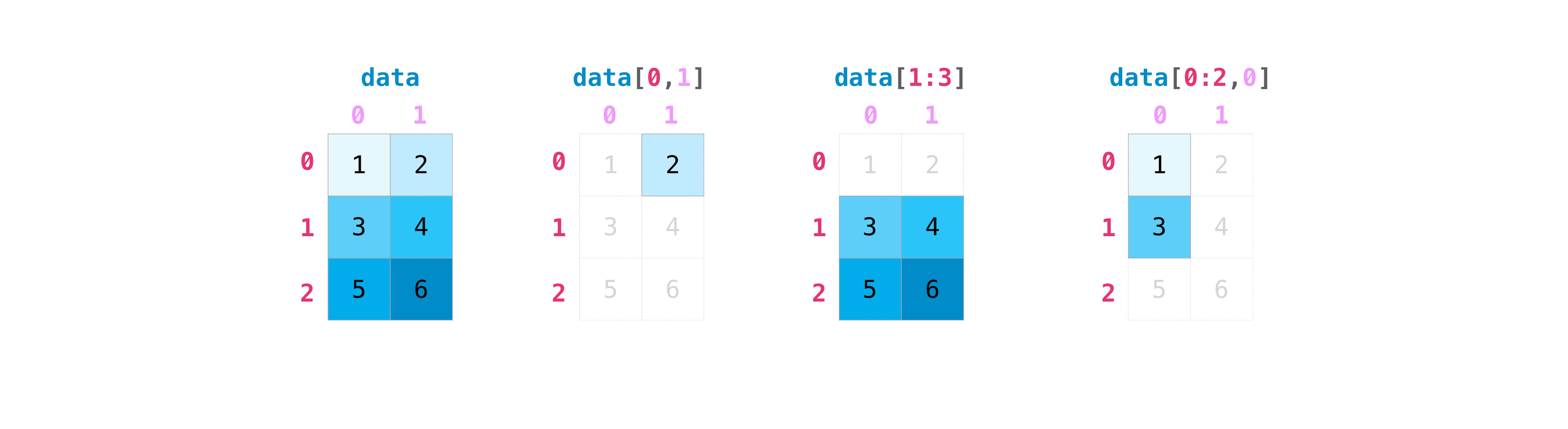
Here are the central patterns:

data[1, 0]      # 3: row 1, column 0
data[1]         # [3, 4]: all columns in row 1
data[:, 0]      # [1, 3, 5]: column 0 from every row
data[1:3, :]    # [[3, 4], [5, 6]]: rows 1 and 2, all columns
data[0:2, 0:1]  # [[1], [3]]: first two rows, first column

The final two examples look similar but have an important difference:

print(data[:, 0].shape)    # (3,)
print(data[:, 0:1].shape)  # (3, 1)

An integer index removes the indexed axis. A slice preserves it, even when the slice selects one position. If downstream code requires a two-dimensional column, data[:, 0:1] is often more appropriate than data[:, 0].

Basic slices usually return a view into the original array rather than an independent copy. That is efficient, but mutation can be surprising:

scores = np.array([0.82, 0.61, 0.94, 0.73])

first_two = scores[:2]
first_two[0] = 0.0

print(scores)
# [0.   0.61 0.94 0.73]

When you need an independent result that you plan to modify, make the decision explicit:

first_two_copy = scores[:2].copy()

Boolean indexing selects by condition

A Boolean array can select observations that meet a condition. This is particularly useful for data checks and slice-based ML evaluation.

latency_ms = np.array([42.1, 85.7, 38.4, 121.5, 63.2])

slow_requests = latency_ms[latency_ms > 80]
print(slow_requests)
# [ 85.7 121.5]

For a feature matrix, a one-dimensional mask aligned with axis 0 selects whole rows:

ages = np.array([16, 25, 31, 14])
adult_X = X[ages >= 18]

print(adult_X.shape)  # (2, 3)

The mask has shape (4,), matching the number of observations in X. It retains the rows for the second and third observations. That shape alignment is the crucial check before applying a Boolean mask.

For multiple conditions, parenthesize each comparison and use element-wise operators:

eligible = (ages >= 18) & (ages < 30)

Do not use Python’s and or or between NumPy Boolean arrays; use & or |.

---

Broadcasting: align shapes from the right

Broadcasting allows NumPy to perform element-wise operations on compatible arrays of different shapes. A scalar is the simplest example:

scores = np.array([0.81, 0.63, 0.94])
percentages = scores * 100

Conceptually, 100 is available at every position. NumPy does not need to build a full copied array of hundreds to do this.

The key rule for two arrays is:

Compare dimensions from the rightmost side. Each pair must be equal, or one of the dimensions must be 1. Missing leading dimensions behave as if they had size 1.

For a matrix A of shape (4, 3) and a feature adjustment vector b of shape (3,):

A = np.array([
    [0, 0, 0],
    [10, 10, 10],
    [20, 20, 20],
    [30, 30, 30],
])

b = np.array([1, 2, 3])

result = A + b
print(result)
# [[ 1  2  3]
#  [11 12 13]
#  [21 22 23]
#  [31 32 33]]

b aligns with the last axis of A, the feature or column axis. Its values are applied to every row.

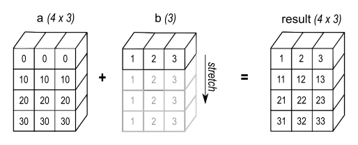
This is why feature-wise normalization works: a vector containing one statistic per feature aligns with a batch matrix’s final, feature dimension.

Read NumPy’s official broadcasting rules. They are concise enough to use as a reference whenever a shape error occurs.

A common error: a per-row vector is not shaped as a column

Suppose you have one adjustment per row:

row_adjustment = np.array([100, 200, 300, 400])

print(A.shape)               # (4, 3)
print(row_adjustment.shape)  # (4,)

This fails:

A + row_adjustment
# ValueError: operands could not be broadcast together ...

NumPy compares the last dimensions first: 3 and 4 do not match, and neither is 1.

If you intend one adjustment for every row, make that intent explicit by inserting a final axis:

row_adjustment = row_adjustment[:, None]

print(row_adjustment.shape)  # (4, 1)

result = A + row_adjustment
print(result)
# [[100 100 100]
#  [210 210 210]
#  [320 320 320]
#  [430 430 430]]

The (4, 1) array supplies one value for each row and broadcasts that value across the three columns.

Conversely, to make a one-row array explicitly, use:

feature_adjustment = np.array([1, 2, 3])[None, :]
print(feature_adjustment.shape)  # (1, 3)

A compact visual summary:

Intended meaning	Appropriate shape with a batch of shape (n, d)
One scalar for everything	()
One value per feature	(d,) or (1, d)
One value per observation	(n, 1)
A separate value for every observation-feature pair	(n, d)

The intended meaning must choose the shape. A reshape that merely silences an error can create a calculation that runs but applies values along the wrong axis. This is especially risky when n and d happen to be equal, because an accidental alignment may produce no error at all.

Broadcasting can create useful grids

Broadcasting can intentionally form combinations. For example, these two vectors define every row-column sum:

row_values = np.array([0, 10, 20, 30])[:, None]  # (4, 1)
column_values = np.array([1, 2, 3])[None, :]     # (1, 3)

grid = row_values + column_values
print(grid.shape)  # (4, 3)

This pattern appears in distance calculations, score matrices, and positional computations. It is powerful, but check the output shape before applying it to large data. Broadcasting often avoids copying small inputs, yet an operation can still create a large output or intermediate array. For example, comparing every item in one large collection with every item in another can require a memory-heavy pairwise result. Concise syntax is not automatically low-memory syntax.

---

A disciplined workflow for dimension errors

When NumPy reports a shape mismatch, do not begin by guessing at reshape. Use this sequence:

1. Print the actual shapes.

   print("X:", X.shape)
   print("mean:", feature_means.shape)
   

2. Name each axis semantically. For example, X may be (batch, features), while a vector might represent (features,) or (batch,). These are different contracts.

3. Work right to left for broadcasting. Compare the final dimensions, then the next pair to the left. A match requires equal sizes or a size of 1.

4. Choose the operation that reflects the intended meaning.

   • Use [:, None] to turn a per-row vector into (batch, 1).
   • Use [None, :] to turn a per-feature vector into (1, features).
   • Use reshape only when regrouping the data is genuinely correct.
   • Use .T only when exchanging axes is genuinely correct.

5. Validate with a tiny, recognizable example. Arrays containing values such as 10, 20, 30 make it easy to see whether a value was applied across rows or columns.

For an immediate compatibility check, NumPy can calculate the broadcasted output shape without performing arithmetic:

A = np.zeros((4, 3))
feature_values = np.array([1, 2, 3])

print(np.broadcast_shapes(A.shape, feature_values.shape))
# (4, 3)

In production ML code, assertions near system boundaries can turn confusing downstream failures into clear messages:

def validate_feature_batch(X, expected_features):
    if X.ndim != 2:
        raise ValueError(f"Expected a 2D batch, got shape {X.shape}")

    if X.shape[1] != expected_features:
        raise ValueError(
            f"Expected {expected_features} features, got shape {X.shape}"
        )

The same habit will matter later in PyTorch, where tensor-shape failures can surface deep inside a model. Inspecting shapes at the data-loading and preprocessing boundaries is much faster than debugging an opaque training-time exception.

---

Key takeaways

A NumPy shape is an ordered description of axes, and in ML it should be treated as a data-interface contract. Use .shape, .ndim, and .size to inspect arrays before assuming what they represent.

reshape changes grouping while preserving element count; transpose reorders axes; None or np.newaxis inserts a dimension of size one. Reductions remove the selected axis unless keepdims=True, so axis=0 on a batch-by-feature array produces one result per feature, while axis=1 produces one result per observation.

For indexing, use comma-separated indices per axis and remember that integer indexing removes an axis while slicing preserves it. For broadcasting, compare shapes from the right: dimensions must match or one must be 1. Choose (n, 1) for per-row values and (1, d) or (d,) for per-feature values.

Next, you will use these array skills to load and inspect structured datasets with pandas, looking for schema and data-quality issues before they become model problems.