SVMs and Kernel Methods

Hello! Let's dive into our next topic.

Introduction

In our previous lessons, we explored two fundamentally different classification algorithms. We started with logistic regression, a discriminative model that learns a decision boundary directly. Then, we examined Naive Bayes, a generative model that learns the probability distribution of the data for each class.

Today, we return to the discriminative family to study one of the most powerful and influential classical algorithms: Support Vector Machines (SVMs). This lesson directly addresses the learning outcome: Apply support vector machines (SVMs) with different kernel methods.

Unlike logistic regression, which finds any reasonable decision boundary, an SVM seeks to find the optimal one. It takes a geometric approach, aiming to identify the hyperplane that has the maximum possible margin, or "street," between the different classes. This principle of maximizing the margin makes the model robust and gives it excellent generalization properties.

We will cover:

1. The core intuition of the maximum margin classifier.
2. How to handle real-world, messy data using the soft-margin SVM with the regularization parameter C.
3. The kernel trick, a brilliant mathematical shortcut that allows SVMs to create complex, non-linear decision boundaries.
4. An exploration of common kernel functions—Linear, Polynomial, and RBF (Gaussian)—and their key hyperparameters.
5. How to apply these concepts in practice using Python's scikit-learn library.

1. The Core Idea: Maximizing the Margin

Imagine you have a set of data points belonging to two classes that are linearly separable. You could draw many possible straight lines (or hyperplanes in higher dimensions) to separate them. Which one is the best?

The core idea of the SVM is to choose the hyperplane that is farthest from the nearest data point of any class. We want to find the line that creates the widest possible "street" between the classes.

The data points that lie on the edges of this street are called support vectors. They are the critical elements of the dataset because they alone "support" or define the position of the optimal hyperplane. If you were to move any of the other data points, the decision boundary wouldn't change. But if you move a support vector, the boundary will likely shift.

This video provides an excellent visual and conceptual introduction to these ideas.

This maximization of the margin is framed as a constrained optimization problem. The goal is to maximize the margin's width, which turns out to be equivalent to minimizing $\frac{1}{2}||\mathbf{w}|{|}^2$, where $\mathbf{w}$ is the vector normal to the hyperplane. The constraints ensure that all data points are classified correctly and lie outside the margin. This is known as the hard-margin SVM.

2. Handling Messy Data: The Soft Margin SVM

The hard-margin SVM works beautifully for perfectly separable data. However, most real-world datasets contain noise and outliers, making a perfect linear separation impossible or undesirable. An SVM that insists on perfect separation might create a very contorted boundary that overfits the training data.

The solution is the soft-margin SVM. We relax the rules and allow some data points to be misclassified or to fall inside the margin. We introduce a "cost" for each violation, and the model's goal becomes a trade-off: keep the margin as wide as possible while keeping the number of margin violations as low as possible.

This trade-off is controlled by a crucial hyperparameter, C (the regularization parameter):

• A high C value puts a high penalty on misclassification. The SVM will try very hard to classify all points correctly, leading to a narrower margin and a more complex decision boundary. This can lead to overfitting.
• A low C value puts a lower penalty on misclassification. The SVM will be more tolerant of errors and will prioritize a wider margin, leading to a simpler decision boundary. This can lead to underfitting.

The following video segments explain how this is achieved with slack variables and the C parameter.

3. The Magic of Kernels for Non-Linear Data

So far, we've only considered linear decision boundaries. But what if our data is fundamentally non-linear, like two concentric circles? No straight line can separate them.

This is where SVMs truly shine, using a technique known as the kernel trick. The idea is to project the data into a higher-dimensional space where it becomes linearly separable.

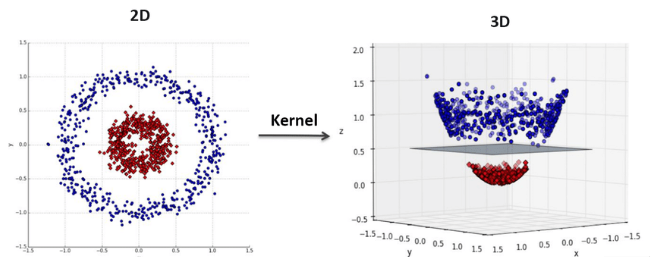
Performing this projection explicitly could be computationally very expensive or even impossible if the target dimension is infinite. The "trick" is that we don't have to. The SVM's optimization problem can be reformulated (into its dual form) so that it only ever needs the dot product of pairs of data vectors, ${\mathbf{x}}_i\cdot {\mathbf{x}}_j$.

A kernel function, $K({\mathbf{x}}_i,{\mathbf{x}}_j)$, is a function that calculates this dot product for us in the higher-dimensional space, without ever explicitly computing the transformation. This is a powerful and efficient shortcut.

The following videos explain this crucial concept from both a conceptual and mathematical perspective.

4. Applying SVMs with Different Kernels

Now that we understand the theory, let's look at how to apply it. The scikit-learn library provides a robust implementation of SVMs. The main class is sklearn.svm.SVC (Support Vector Classifier).

When creating an SVC object, you can specify the kernel function and its parameters. Let's look at the most common ones.

Here's a summary of the key kernels:

• Linear Kernel: kernel='linear'

  • Formula: $K({\mathbf{x}}_i,{\mathbf{x}}_j)={\mathbf{x}}_i^T{\mathbf{x}}_j$
  • This is the standard SVM without any non-linear transformation. It's fast and a good baseline.

• Polynomial Kernel: kernel='poly'

  • Formula: $K({\mathbf{x}}_i,{\mathbf{x}}_j)=(\gamma {\mathbf{x}}_i^T{\mathbf{x}}_j+r{)}^d$
  • Key Hyperparameters:
    • degree (d): The degree of the polynomial. Higher degrees create more flexible boundaries.
    • gamma: A coefficient scaling the dot product.
    • coef0 (r): An independent term.

• Radial Basis Function (RBF) Kernel: kernel='rbf'

  • Formula: $K({\mathbf{x}}_i,{\mathbf{x}}_j)=\exp (-\gamma ||{\mathbf{x}}_i-{\mathbf{x}}_j|{|}^2)$
  • This is often the default and most popular choice. It can model very complex regions.
  • Key Hyperparameter:
    • gamma: Defines the influence of a single training example. A small gamma means a point has a large influence (smoother boundary), while a large gamma means a point has a small, localized influence (more complex, wiggly boundary).

The choice of C and the kernel-specific parameters like gamma and degree is critical. Finding the right combination, often via techniques like Grid Search with cross-validation, is key to an SVM's performance.

Practical Implementation in scikit-learn

Here is how you would train SVMs with different kernels in Python:

from sklearn import svm
from sklearn.datasets import make_circles
from sklearn.model_selection import train_test_split

# Create a non-linear dataset
X, y = make_circles(n_samples=100, factor=0.5, noise=0.1, random_state=42)
X_train, X_test, y_train, y_test = train_test_split(X, y, random_state=42)

# 1. Linear SVM
linear_svm = svm.SVC(kernel='linear', C=1.0)
linear_svm.fit(X_train, y_train)
print(f"Linear SVM Score: {linear_svm.score(X_test, y_test):.2f}")

# 2. RBF SVM
rbf_svm = svm.SVC(kernel='rbf', gamma=2, C=1.0) # Try changing gamma and C
rbf_svm.fit(X_train, y_train)
print(f"RBF SVM Score: {rbf_svm.score(X_test, y_test):.2f}")

# 3. Polynomial SVM
poly_svm = svm.SVC(kernel='poly', degree=3, C=1.0)
poly_svm.fit(X_train, y_train)
print(f"Polynomial SVM Score: {poly_svm.score(X_test, y_test):.2f}")

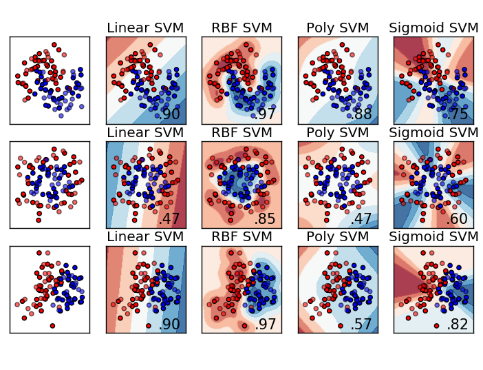
Running this code, you'll see that the RBF kernel performs best on this circular dataset, as expected.

Conclusion

In this lesson, we explored the powerful and elegant Support Vector Machine algorithm. Starting from a simple geometric intuition, we built up to a sophisticated classifier capable of handling complex, non-linear problems.

Key Takeaways:

• SVMs are discriminative classifiers that find the optimal hyperplane by maximizing the margin between classes.
• The decision boundary is defined by a small subset of the data called support vectors.
• The soft-margin SVM uses the regularization parameter C to balance the trade-off between maximizing the margin and minimizing classification errors, making it robust to noise and outliers.
• The kernel trick allows SVMs to create complex, non-linear decision boundaries by implicitly mapping data to a higher-dimensional space.
• Common kernels include Linear, Polynomial, and RBF (Gaussian), each with its own hyperparameters (degree, gamma) that control the flexibility of the model.

Preview of the next lesson:
We have now studied three major approaches to classification: probabilistic (Naive Bayes), linear/optimization-based (Logistic Regression), and geometric/margin-based (SVM). Next, we will explore a completely different paradigm: Decision Trees. These models make predictions by learning a hierarchy of simple if/then/else questions, creating a tree-like structure that is highly interpretable. This will serve as a crucial building block for some of the most powerful algorithms in machine learning, such as Random Forests and Gradient Boosting.