Exploring NumPy Arrays, Shapes, Axes, and Data Types

Welcome to Month 1. This first module builds the numerical vocabulary you will use throughout the course: NumPy arrays, vectors, matrices, derivatives, probability, and visual inspection of data. Today’s micro-challenge establishes a habit that prevents many downstream machine-learning bugs: whenever you create data, inspect its number of axes, shape, and data type before operating on it.

By the end, you will be able to construct one-dimensional and two-dimensional NumPy arrays, explain what each axis represents, and verify an array’s structure with ndim, shape, size, and dtype. Plan for about 35–40 minutes, including the implementation task.

---

Arrays are structured numerical data

NumPy’s core object is an ndarray: an N-dimensional array. Its main advantage is that it stores values in a regular, homogeneous structure: every element has one data type, and two-dimensional data must be rectangular rather than jagged.

For this course, begin with two useful cases:

• A one-dimensional array has one axis: a sequence of values.
• A two-dimensional array has two axes: commonly interpreted as rows and columns.

For example:

import numpy as np

temperatures = np.array([12, 15, 14, 18])
sales = np.array([[120.5, 98.0, 110.0],
                  [130.0, 105.5, 125.0]])

temperatures is one-dimensional. Its four values sit along a single axis.

sales is two-dimensional. It has two rows and three columns. In most tabular machine-learning datasets, the convention will be:

• Axis 0: rows, usually observations or records.
• Axis 1: columns, usually features or variables.

That convention is meaningful because we assign it meaning. NumPy itself only sees axes in positional order: first axis, second axis, and so on.

---

Reading an array’s structural metadata

The following four attributes are the basic “identity card” for an array. They are attributes, not functions, so write array.shape, not array.shape().

Attribute	Meaning	Example for a $2\times 3$ array
ndim	Number of axes	2
shape	Length along each axis	(2, 3)
size	Total number of elements	6
dtype	Data type shared by elements	float64, int16, etc.

The key relationship is:

$$\text{size}=\prod \text{shape dimensions}$$

So an array with shape == (2, 3) contains $2\cdot 3=6$ values.

A frequent beginner confusion is between these two objects:

np.array([1, 2, 3, 4])      # shape (4,), one axis
np.array([[1, 2, 3, 4]])    # shape (1, 4), two axes

They contain the same number of values but have different structures. The first is a one-dimensional vector-like array; the second has one row and four columns. Later, that difference will affect broadcasting, matrix operations, model inputs, and plotting.

The supplied NumPy reshape image makes the distinction between shape and data especially concrete.

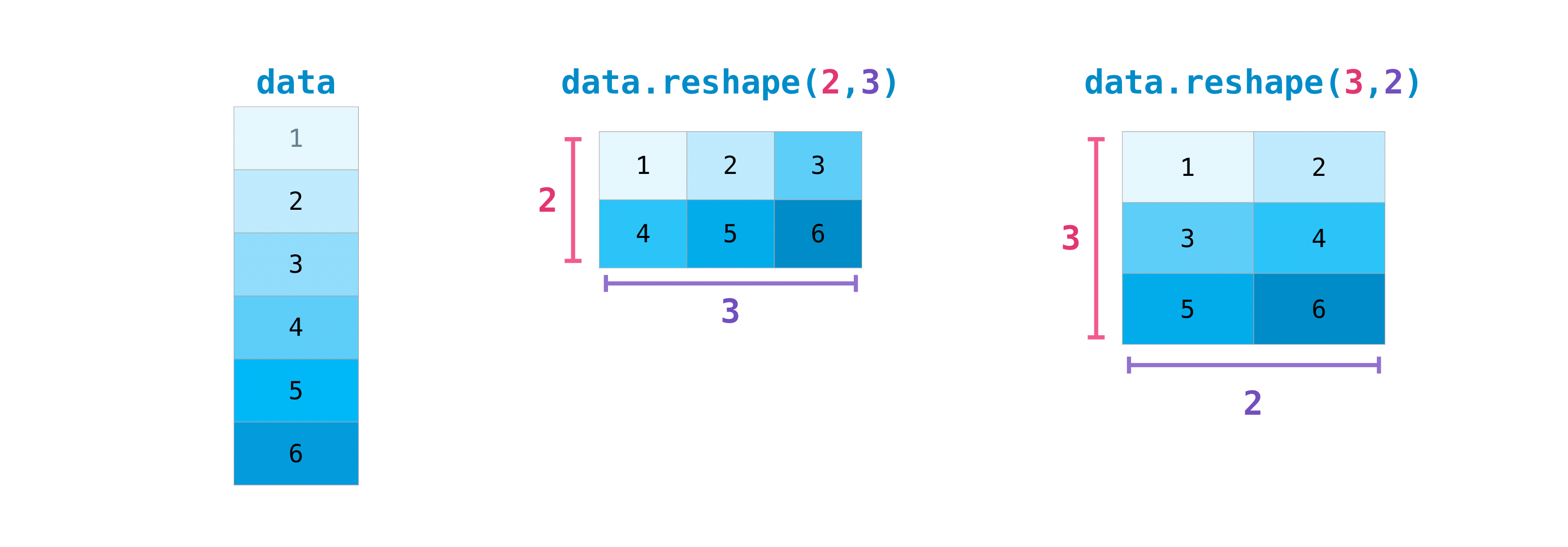
You will use reshape formally in a later NumPy lesson. For now, use the image to reinforce the main point: a shape tells NumPy how values are organized across axes.

---

Concept-Level Micro-Challenge: construct, inspect, and explain

Open a new notebook or Python file. Type and run the following 13-line NumPy program rather than pasting it blindly. It deliberately uses explicit data types so that your output is reproducible across machines.

import numpy as np
temperatures = np.array([12, 15, 14, 18], dtype=np.int16)
sales = np.array(
    [[120.5, 98.0, 110.0],
     [130.0, 105.5, 125.0]], dtype=np.float64)
for name, arr in {"temperatures": temperatures, "sales": sales}.items():
    print(f"\n{name}")
    print("ndim:", arr.ndim)
    print("shape:", arr.shape)
    print("size:", arr.size)
    print("dtype:", arr.dtype)
print("\nsales axis 0 =", sales.shape[0], "rows")
print("sales axis 1 =", sales.shape[1], "columns")

Your essential checks are:

• temperatures reports:

  • ndim: 1
  • shape: (4,)
  • size: 4
  • dtype: int16

• sales reports:

  • ndim: 2
  • shape: (2, 3)
  • size: 6
  • dtype: float64

Interpret the result in data terms:

• temperatures.shape == (4,) means one axis containing four daily temperature values.
• sales.shape == (2, 3) means axis 0 has two records and axis 1 has three values per record.
• sales.size == 6 verifies that two rows times three columns gives six stored values.
• dtype is intentional: counts or compact integer values may fit an integer type, while measurements such as sales amounts often require floating-point values.

A useful debugging routine is to print these attributes immediately after loading or transforming data. If you expected 500 records with 12 features, but see (12, 500) or (6000,), inspect the structure before training a model. A correct-looking set of values can still be arranged incorrectly.

---

Why dtype deserves attention

NumPy arrays are normally homogeneous. This means one array has one element type, unlike a Python list that can mix an integer, a string, and a Boolean value without complaint.

np.array([1, 2, 3])          # typically an integer dtype
np.array([1.0, 2.5, 3.0])    # floating-point dtype
np.array([1, 2.5, 3])        # values are promoted to a floating dtype

For the micro-challenge, dtype=np.int16 and dtype=np.float64 tell NumPy exactly how to store the data. At this stage, the important practical rule is not “always choose the smallest type.” It is:

Choose a type that represents the data correctly, and inspect it when results look surprising.

For example, a column containing missing values will often need a floating-point representation even if its non-missing values look like integers. You will encounter this issue again when cleaning tabular data in Pandas.

---

Takeaways

A NumPy array is structured numerical data, described by its axes and its shared data type.

• A one-dimensional array has one axis; its shape looks like (n,).
• A two-dimensional array has two axes; its shape looks like (rows, columns).
• ndim counts axes, shape gives each axis length, size counts all elements, and dtype identifies the stored element type.
• In tabular ML data, axis 0 is conventionally observations and axis 1 is features—but always verify this assumption with shape.

Next, you will use these arrays for actual numerical operations: vector addition, scalar multiplication, and Euclidean norms.