Directed Cohort Connectivity: Synapse Counts and Degree Summaries

Welcome back. Your capstone now has a validated primary cohort: every included neuron has a documented annotation basis, a bounded morphology review, and a fixed materialization context. That means you can calculate connectivity without silently mixing uncertain candidates into the central result.

In this lesson, you will turn that cohort into a directed, weighted network: each row in the core edge table will represent presynaptic neuron, postsynaptic neuron, and the number of filtered synapses joining them. You will also produce per-neuron summaries of incoming and outgoing synapse totals and partner counts, with the query settings saved alongside the outputs.

Plan for roughly 40 minutes: about 8 minutes reading the API contract, 25 minutes implementing the notebook cells, and 7 minutes checking and exporting results.

---

What “directed cohort connectivity” means

A synapse has a direction. In FlyWire connectivity data:

• a source is the presynaptic neuron;
• a target is the postsynaptic neuron;
• an edge’s weight is the number of synapses observed from that source to that target under the chosen filtering and materialization settings.

For a cohort of $n$ neurons, represent internal connectivity as an adjacency matrix $A$, where rows are sources and columns are targets:

$$A_{ij}=\text{number of filtered synapses from cohort neuron }i\text{ to cohort neuron }j$$

A nonzero $A_{ij}$ does not imply that $A_{ji}$ is nonzero. Reciprocal connectivity must be measured, not assumed.

The full matrix is convenient for computation, but the canonical analysis result should be a long-form edge table:

source_root_id	target_root_id	synapse_count
720575940...	720575940...	18
720575940...	720575940...	4

This format works well with pandas, NetworkX, CSV exports, and the visualization work in the next lesson.

The FlyWire interface can show connectivity in several complementary forms: EM evidence, 3D reconstructions, connection graphs, and tabular partner data.

---

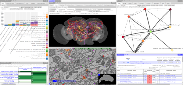
Read the query contract before writing analysis code

The most important choice here is not a plotting library or a graph metric. It is making the scope of the query explicit: which root IDs, which materialization, and which synapse filtering rule.

For this capstone, use get_adjacency, rather than querying every partner in the whole brain and filtering afterward. The former asks a narrow, auditable question:

Among the neurons in this validated cohort, how many filtered synapses connect each ordered source-target pair?

This is a cohort-internal network. It does not say how many total synapses each neuron receives from or sends to the entire brain. Keep those two scopes distinct in filenames and interpretation.

---

Load only the validated primary cohort

Reuse the materialization version and dataset context that you fixed in the earlier notebook. Do not use "latest", "auto", or "live" for the capstone result: each can cause results to change or choose a different version than the one used for cohort selection.

The code below assumes you have a small JSON provenance file from the earlier lessons. Adapt only the file path or field names if your project uses a different layout; do not substitute a newly discovered materialization version.

from datetime import datetime, timezone
from pathlib import Path
import json

import numpy as np
import pandas as pd
from fafbseg import flywire

# This file should contain values already pinned in your earlier notebook.
# Expected keys: "dataset" and "materialization_version".
project = json.loads(
    Path("data/derived/project_provenance.json").read_text()
)

DATASET = project["dataset"]
MATERIALIZATION = int(project["materialization_version"])

validation = pd.read_csv(
    "data/derived/cohort_validation.csv",
    dtype={"root_id": "string"}
)

# Primary analysis is limited to neurons explicitly reviewed and included.
primary = validation.loc[
    (validation["decision"] == "included")
    & (validation["analysis_role"] == "primary")
].copy()

if primary.empty:
    raise ValueError("No primary cohort members found.")

if primary["root_id"].isna().any():
    raise ValueError("Primary cohort contains a missing root ID.")

if primary["root_id"].duplicated().any():
    raise ValueError("Primary cohort contains duplicate root IDs.")

cohort_ids_text = primary["root_id"].astype("string").tolist()
cohort_ids = [int(root_id) for root_id in cohort_ids_text]

print(f"Dataset: {DATASET}")
print(f"Materialization: {MATERIALIZATION}")
print(f"Primary cohort size: {len(cohort_ids)}")
display(primary)

Root IDs are stored as text in CSV outputs because they are large identifiers, not quantities you intend to add or average. They are converted to Python integers only at the point where the FlyWire query requires them.

Before proceeding, inspect the displayed primary table. It should contain exactly the neurons you intended to retain after the annotation and morphology-validation lesson. If an unresolved candidate appears here, stop and correct cohort_validation.csv; do not patch the list manually in a later cell.

---

Query the weighted internal adjacency matrix

Now request connectivity with the primary cohort as both the sources and targets.

adjacency = flywire.get_adjacency(
    sources=cohort_ids,
    targets=cohort_ids,
    square=True,
    materialization=MATERIALIZATION,
    filtered=True,
    min_score=None,
    neuropils=False,
    batch_size=1000,
    dataset=DATASET,
    progress=True,
)

# Preserve the cohort's documented ordering and make CSV labels unambiguous.
adjacency = adjacency.reindex(index=cohort_ids, columns=cohort_ids, fill_value=0)
adjacency = adjacency.astype("int64")

adjacency.index = pd.Index(cohort_ids_text, name="source_root_id")
adjacency.columns = pd.Index(cohort_ids_text, name="target_root_id")

display(adjacency)

The resulting table has an important invariant:

• Its rows are presynaptic source IDs.
• Its columns are postsynaptic target IDs.
• Each value is a filtered synapse count.

For example, if the row for neuron A and column for neuron B contains 12, then this materialization contains 12 filtered synapses from A to B within the query’s connectivity table.

A zero means that no filtered synapses were returned for that ordered pair. It does not prove that the two neurons never interact biologically; it is conditional on reconstruction state, synapse detection, filtering, and the selected data release.

Convert the matrix into the directed edge table

Most downstream analyses should use a table containing only observed edges.

edge_table = (
    adjacency
    .rename_axis(index="source_root_id", columns="target_root_id")
    .stack()
    .rename("synapse_count")
    .reset_index()
)

# Keep only observed connections within the cohort.
edge_table = edge_table.loc[
    edge_table["synapse_count"] > 0
].copy()

# Preserve self-connections, if present, but label them explicitly.
edge_table["is_autapse"] = (
    edge_table["source_root_id"] == edge_table["target_root_id"]
)

edge_table = edge_table.sort_values(
    ["synapse_count", "source_root_id", "target_root_id"],
    ascending=[False, True, True],
    kind="stable",
).reset_index(drop=True)

display(edge_table.head(20))

At this point, you have fulfilled the central data product of the lesson: a directed cohort-connectivity table in which each row is one source-target pair and synapse_count is its edge weight.

---

Calculate weighted and unweighted in-degree and out-degree

“In-degree” and “out-degree” can mean two different things in a weighted synaptic network. Reporting both avoids ambiguity.

For neuron $i$, define its weighted outgoing synapse total and weighted incoming synapse total as:

$$s_i^{\mathrm{out}}=\sum _{j\ne i}{A}_{ij}$$ $$s_i^{\mathrm{in}}=\sum _{j\ne i}{A}_{ji}$$

These are counts of synapses connecting the neuron to other members of the cohort.

Also calculate outgoing partner count and incoming partner count. These are conventional unweighted degrees: each connected partner counts once, regardless of whether the pair has one synapse or one hundred.

For the principal cohort-network summary, exclude autapses from degree calculations. Autapses remain in the edge table and are reported separately, rather than being silently discarded.

# Use a copy so the raw adjacency matrix remains unchanged.
adjacency_no_self = adjacency.copy()
np.fill_diagonal(adjacency_no_self.values, 0)

# Start with reviewed cohort metadata, retaining useful labels if present.
summary = (
    primary.assign(root_id=primary["root_id"].astype("string"))
    .drop_duplicates("root_id")
    .set_index("root_id")
    .reindex(cohort_ids_text)
    .copy()
)

summary.index.name = "root_id"

# Weighted degrees: counts of cohort-internal synapses.
summary["outgoing_synapses_within_cohort"] = (
    adjacency_no_self.sum(axis=1).to_numpy()
)

summary["incoming_synapses_within_cohort"] = (
    adjacency_no_self.sum(axis=0).to_numpy()
)

# Unweighted degrees: counts of distinct cohort partners.
summary["outgoing_partners_within_cohort"] = (
    (adjacency_no_self > 0).sum(axis=1).to_numpy()
)

summary["incoming_partners_within_cohort"] = (
    (adjacency_no_self > 0).sum(axis=0).to_numpy()
)

# Optional but useful: identify autapses separately.
autapse_counts = pd.Series(
    np.diag(adjacency.values),
    index=adjacency.index,
    name="autapse_synapses",
)

summary = summary.join(autapse_counts)

summary = summary.sort_values(
    "outgoing_synapses_within_cohort",
    ascending=False,
    kind="stable",
)

display(
    summary[
        [
            "outgoing_synapses_within_cohort",
            "incoming_synapses_within_cohort",
            "outgoing_partners_within_cohort",
            "incoming_partners_within_cohort",
            "autapse_synapses",
        ]
    ]
)

Use the names literally in your notebook and exported files. For example:

• outgoing_synapses_within_cohort is a weighted out-degree summary.
• outgoing_partners_within_cohort is an unweighted out-degree summary.
• Neither quantity is the neuron’s whole-brain output.

That last distinction is especially important for small cohorts. A neuron with only a few cohort-internal synapses may still have a large total output elsewhere in the brain.

---

Check the table like a data contract

Before exporting, run a few checks. This is similar to validating an API response: the values themselves may be scientifically interesting, but the object also has structural invariants that should always hold.

# Every primary cohort neuron must appear once as a row and once as a column.
assert list(adjacency.index) == cohort_ids_text
assert list(adjacency.columns) == cohort_ids_text

# No negative synapse counts are meaningful.
assert (adjacency.to_numpy() >= 0).all()

# Long-form edges must reproduce the nonzero matrix entries.
nonzero_weight_from_edges = edge_table["synapse_count"].sum()
nonzero_weight_from_matrix = adjacency.to_numpy().sum()

assert nonzero_weight_from_edges == nonzero_weight_from_matrix

# After excluding autapses, total outgoing and incoming weight must match.
internal_weight = adjacency_no_self.to_numpy().sum()

assert summary["outgoing_synapses_within_cohort"].sum() == internal_weight
assert summary["incoming_synapses_within_cohort"].sum() == internal_weight

print(f"Observed directed cohort edges: {len(edge_table)}")
print(f"All cohort-internal synapses, including autapses: {nonzero_weight_from_matrix}")
print(f"Cohort-internal synapses, excluding autapses: {internal_weight}")
print(f"Autapse edges: {edge_table['is_autapse'].sum()}")

Do not assert that the cohort must contain at least one edge. An empty internal network can be a valid result for a narrowly selected cohort. It would, however, deserve a careful interpretation: the selection rule may have isolated neurons that mainly connect outside the group.

A strong output table also makes directional asymmetry visible. If neuron A has 80 outgoing synapses to B, while B has 2 outgoing synapses to A, that is not an inconsistency. It is the kind of directed structure your next visualization should preserve.

---

Export analysis-ready files with provenance

Save both matrix and edge-list forms. The matrix is convenient for quick inspection; the edge list is the durable analysis product.

output_dir = Path("data/derived")
output_dir.mkdir(parents=True, exist_ok=True)

adjacency.to_csv(
    output_dir / "cohort_adjacency_matrix.csv",
    index_label="source_root_id",
)

edge_table.to_csv(
    output_dir / "cohort_connectivity_edges.csv",
    index=False,
)

summary.reset_index().to_csv(
    output_dir / "cohort_connectivity_node_summary.csv",
    index=False,
)

provenance = {
    "dataset": DATASET,
    "materialization_version": MATERIALIZATION,
    "cohort_source": "data/derived/cohort_validation.csv",
    "cohort_rule": (
        "decision == included and analysis_role == primary"
    ),
    "cohort_root_ids": cohort_ids_text,
    "query_method": "fafbseg.flywire.get_adjacency",
    "synapse_filtering": (
        "filtered=True, min_score=None, neuropils=False"
    ),
    "edge_scope": "directed connections among primary cohort members only",
    "autapse_handling": (
        "Retained and flagged in edge table; excluded from degree summaries."
    ),
    "queried_at_utc": datetime.now(timezone.utc).isoformat(),
}

with open(output_dir / "cohort_connectivity_provenance.json", "w") as f:
    json.dump(provenance, f, indent=2)

print("Saved:")
for path in sorted(output_dir.glob("cohort_*connectivity*")):
    print(" -", path)

Your output directory should now contain:

File	Purpose
cohort_connectivity_edges.csv	Canonical directed, weighted edge table
cohort_adjacency_matrix.csv	Square source-by-target matrix
cohort_connectivity_node_summary.csv	Weighted and unweighted incoming/outgoing summaries
cohort_connectivity_provenance.json	Query scope, filtering, materialization, and autapse convention

Keep the original cohort_validation.csv alongside these files. It explains why particular root IDs are represented in the network at all.

---

Wrap-up

You now have a reproducible, directed cohort-connectivity dataset:

• each edge represents a presynaptic source, a postsynaptic target, and a filtered synapse count;
• the matrix and long-form edge table describe the same cohort-internal network;
• weighted summaries count synapses, while unweighted summaries count distinct partners;
• autapses are preserved as evidence but excluded from the main degree summaries by an explicit convention;
• the materialization version, query settings, and exact cohort IDs are recorded with the outputs.

Next, you will turn these tables into a visualization that communicates the cohort’s strongest directed connections without hiding directionality, connection weight, or uncertainty.