NumPy Indexing, Vectorization, and Broadcasting

Good to see you again. In the previous lesson, you used generators to move text through a pipeline without loading an entire corpus into memory. That pattern handles when records are consumed. NumPy handles the complementary problem: once a numerical batch is in memory, it lets you transform many values at once using compact, shape-aware operations.

In this lesson, you will use NumPy arrays to select and filter data with indexing, replace Python loops with vectorized operations, and predict when arrays of different shapes can work together through broadcasting. These are core habits for later work with token batches, embeddings, logits, and gradients.

Plan for about 40–45 minutes: 7 minutes of video, 12–15 minutes of documentation, and 20 minutes working through the code.

---

1. The working model: arrays, axes, and shapes

Import NumPy by convention as np:

import numpy as np

A NumPy ndarray is a fixed-size, rectangular block of values with a single data type. It is not a replacement for every Python collection. Use a list or dictionary for heterogeneous application objects; use an array when you have dense numerical data and want bulk computation.

token_scores = np.array(
    [
        [0.2, 0.8, 0.1, 0.4, 0.5],
        [0.3, 0.7, 0.6, 0.2, 0.1],
        [0.9, 0.2, 0.4, 0.6, 0.3],
        [0.5, 0.1, 0.8, 0.7, 0.2],
    ],
    dtype=np.float32,
)

print(token_scores.shape)  # (4, 5)
print(token_scores.ndim)   # 2
print(token_scores.dtype)  # float32

The shape (4, 5) means:

• axis 0 has length 4: four rows, often interpreted as examples in a batch;
• axis 1 has length 5: five values per example.

Later, model tensors will use more axes. For example, a batch of token IDs often has shape (batch_size, sequence_length), and a batch of token embeddings often has shape (batch_size, sequence_length, embedding_dimension). The interpretation changes with the task; the operational rule does not: read a shape from left to right, and track what each axis represents.

The NumPy documentation’s introductory sections are worth reading once now, particularly for the distinction between array slices and Python-list slices.

---

2. Basic indexing and slicing: select without looping

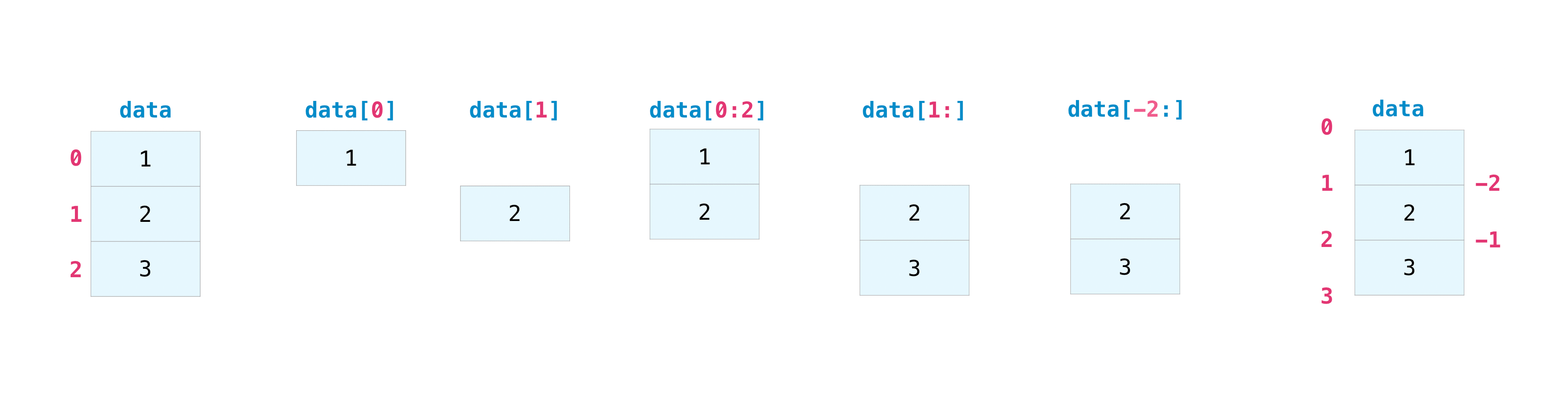
NumPy uses the same zero-based indexing and end-exclusive slicing rules as Python sequences. The difference is that a multidimensional array lets you specify one selector per axis, separated by commas.

scores = np.arange(20).reshape(4, 5)

print(scores)
# [[ 0  1  2  3  4]
#  [ 5  6  7  8  9]
#  [10 11 12 13 14]
#  [15 16 17 18 19]]

For this (4, 5) array:

Expression	Meaning	Result shape
scores[1, 3]	One value: row 1, column 3	scalar
scores[1]	The complete second row	(5,)
scores[:, 2]	The third column from every row	(4,)
scores[1:3, 2:5]	Rows 1–2 and columns 2–4	(2, 3)
scores[:, -1]	Final column from every row	(4,)
scores[::2, ::2]	Every second row and column	(2, 3)

A colon means “all positions along this axis.” Therefore:

second_row = scores[1, :]
third_column = scores[:, 2]

print(second_row)   # [5 6 7 8 9]
print(third_column) # [ 2  7 12 17]

The shorthand scores[1] is equivalent to scores[1, :] here. In production numerical code, however, making the relevant axis explicit can improve readability once tensors have three or four dimensions.

Slicing usually returns a view

Basic slicing does not normally allocate a separate data buffer. It creates a view into the same underlying memory:

window = scores[:2, :3]

window[0, 0] = 999

print(scores[0, 0])  # 999

This can be efficient: extracting a small window is cheap. But it is also a source of accidental mutation. If you need an independent array, make that intention explicit:

safe_window = scores[:2, :3].copy()
safe_window[0, 0] = -1

print(scores[0, 0])  # still 999

A useful default is:

• use a slice view when you deliberately want to work with part of the original array;
• use .copy() at a boundary where the result must become independent.

---

3. Advanced indexing: selecting arbitrary rows and filtering values

Basic slicing selects a regular range. Real data work often needs noncontiguous rows, shuffled examples, or records meeting a condition. NumPy supports this through integer-array indexing and Boolean indexing.

Integer-array indexing

An integer array or Python list can select arbitrary positions:

batch = np.arange(24).reshape(4, 6)

selected = batch[[3, 0, 3]]

print(selected)
# [[18 19 20 21 22 23]
#  [ 0  1  2  3  4  5]
#  [18 19 20 21 22 23]]

This is useful for reordering a batch, selecting sampled examples, or applying the same shuffle indices to aligned arrays:

indices = np.array([2, 0, 3])

features = np.array(
    [
        [0.1, 0.2],
        [0.3, 0.4],
        [0.5, 0.6],
        [0.7, 0.8],
    ]
)
labels = np.array([1, 0, 1, 0])

shuffled_features = features[indices]
shuffled_labels = labels[indices]

Both arrays must use the same indices; otherwise feature rows and labels no longer correspond.

One important distinction: multiple integer index arrays select paired coordinates, not a rectangular region.

grid = np.arange(16).reshape(4, 4)

print(grid[[0, 2], [1, 3]])  # [1, 11]

This selects grid[0, 1] and grid[2, 3]. If you intended all combinations of rows [0, 2] and columns [1, 3], use np.ix_:

corners = grid[np.ix_([0, 2], [1, 3])]

print(corners)
# [[ 1  3]
#  [ 9 11]]

Unlike basic slicing, integer-array indexing creates a copy. That is generally the correct behavior for a gathered or reordered batch.

Boolean indexing: filter with a mask

A Boolean mask is an array of True and False values. Comparisons produce masks element by element:

lengths = np.array([14, 512, 777, 35, 128])

within_limit = lengths <= 512

print(within_limit)
# [ True  True False  True  True]

valid_lengths = lengths[within_limit]

print(valid_lengths)  # [ 14 512  35 128]

This is the NumPy counterpart to filtering a Python collection, but it operates on an entire numerical array in one expression.

For multiple conditions, use & for element-wise “and,” | for element-wise “or,” and ~ for negation. Parenthesize each comparison:

scores = np.array([0.12, 0.91, 0.48, 0.72, 0.03])

keep = (scores >= 0.4) & (scores < 0.9)

print(scores[keep])  # [0.48 0.72]

Do not write this:

# Incorrect for NumPy arrays:
# keep = scores >= 0.4 and scores < 0.9

Python’s and expects one overall truth value, whereas a NumPy comparison produces many truth values. The same warning applies to or.

Masks also support targeted assignment:

losses = np.array([0.4, np.nan, 1.2, np.nan], dtype=np.float32)

losses[np.isnan(losses)] = 0.0

print(losses)  # [0.4 0.  1.2 0. ]

This style will later be useful for identifying padded positions, selecting valid tokens, and masking out values that should not contribute to a calculation.

---

4. Vectorization: express the numerical operation, not the loop

Vectorization means applying an operation to whole arrays rather than iterating through individual elements in Python.

Consider rescaling a collection of numeric features:

values = np.array([2.0, 4.0, 6.0, 8.0], dtype=np.float32)

scaled = values / 2.0
squared = values ** 2
activated = np.maximum(values - 5.0, 0.0)

print(scaled)    # [1. 2. 3. 4.]
print(squared)   # [ 4. 16. 36. 64.]
print(activated) # [0. 0. 1. 3.]

Each expression applies element by element. NumPy implements these operations in optimized native code, rather than repeatedly invoking the Python interpreter for each value. Its homogeneous array representation and low-level numerical kernels are why this is often much faster and more memory-efficient than manipulating a large list of Python numbers.

A Python loop is not inherently wrong. Use one where each iteration has complicated control flow, I/O, or object-level logic. But for dense numerical transformations, first ask whether the operation can be expressed with array arithmetic, comparisons, reductions, or indexing.

Element-wise multiplication is not matrix multiplication

In NumPy, * is element-wise multiplication:

a = np.array([2, 3, 4])
b = np.array([10, 20, 30])

print(a * b)  # [20 60 120]

Matrix multiplication uses @ or np.matmul. You will study the linear-algebra interpretation in the next module; for now, remember that * and @ mean fundamentally different operations.

Reductions and the meaning of axis

Methods such as .sum(), .mean(), .max(), and .std() combine values. Without an axis, they reduce the entire array to one scalar:

features = np.array(
    [
        [1.0, 2.0, 3.0],
        [4.0, 5.0, 6.0],
        [7.0, 8.0, 9.0],
    ]
)

print(features.mean())  # 5.0

With an axis, NumPy removes that axis:

column_means = features.mean(axis=0)
row_means = features.mean(axis=1)

print(column_means)  # [4. 5. 6.]
print(row_means)     # [2. 5. 8.]

axis=0 means “combine down the rows,” leaving one value per column. axis=1 means “combine across columns,” leaving one value per row. This convention can initially feel reversed because axis=0 is the row axis that disappears. The reliable habit is to ask: which axis should be removed?

---

5. Broadcasting: compatible shapes work together

Broadcasting lets NumPy perform element-wise operations between arrays with different shapes when their axes are compatible.

The most common example is adding one feature-wise offset to every row:

features = np.array(
    [
        [10.0, 20.0, 30.0],
        [40.0, 50.0, 60.0],
        [70.0, 80.0, 90.0],
        [15.0, 25.0, 35.0],
    ]
)  # shape: (4, 3)

bias = np.array([0.5, -1.0, 2.0])  # shape: (3,)

adjusted = features + bias

print(adjusted)
# [[10.5 19.  32. ]
#  [40.5 49.  62. ]
#  [70.5 79.  92. ]
#  [15.5 24.  37. ]]

Conceptually, bias is used once for each row. NumPy normally does not need to materialize four physical copies of bias; broadcasting is primarily a shape interpretation used by the operation.

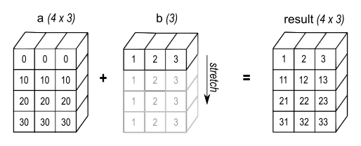
Watch the following explanation before memorizing rules. It gives the most useful mental model: align shapes on the right, then determine which dimensions can expand.

The three broadcasting rules

To compare two shapes:

1. Align their shapes from the right.
2. For each aligned pair of dimensions, the dimensions must either be equal or one must be 1.
3. The output uses the non-one dimension at each position.

For the earlier addition:

features: (4, 3)
bias:        (3)

Treat the shorter shape as though it had a leading dimension of 1:

features: (4, 3)
bias:     (1, 3)
result:   (4, 3)

The final dimension matches: 3 and 3. The first dimension is 4 and 1, so the size-one dimension can broadcast to length four.

A scalar has shape (), so it broadcasts to every element:

normalized = features / 10.0

Row vectors and column vectors are different

A one-dimensional array of shape (4,) is neither explicitly a row nor a column. Its position is determined only after right alignment.

Suppose you want to subtract one offset from every row:

row_offsets = np.array([10.0, 20.0, 30.0, 40.0])  # shape: (4,)

This fails with features, whose shape is (4, 3):

# features - row_offsets
# ValueError: operands could not be broadcast together

After right alignment, NumPy sees (4, 3) and (1, 4). The final dimensions, 3 and 4, conflict.

Add a length-one second axis with None or np.newaxis:

row_offsets_column = row_offsets[:, None]

print(row_offsets_column.shape)  # (4, 1)

row_adjusted = features - row_offsets_column

print(row_adjusted)
# [[ 0. 10. 20.]
#  [20. 30. 40.]
#  [40. 50. 60.]
#  [-25. -15.  -5.]]

Now the shapes are (4, 3) and (4, 1). Each row’s single offset broadcasts across its three columns.

This distinction is central in ML code:

Intent	Typical data shape	Adjustment shape
Apply one value everywhere	(B, D)	scalar ()
Apply one value per feature	(B, D)	(D,)
Apply one value per example	(B, D)	(B, 1)
Apply one value per token position	(B, T, D)	(B, T, 1)

Here, B denotes batch size, T sequence length, and D a feature or embedding dimension.

keepdims=True preserves broadcastable axes

A common need is to reduce an axis and then combine the result back with the original array. keepdims=True retains the reduced axis with length one, making the result broadcastable.

activations = np.array(
    [
        [2.0, 4.0, 6.0, 8.0],
        [10.0, 12.0, 14.0, 16.0],
    ]
)  # shape: (2, 4)

row_mean = activations.mean(axis=1, keepdims=True)

print(row_mean.shape)  # (2, 1)

centered = activations - row_mean

print(centered)
# [[-3. -1.  1.  3.]
#  [-3. -1.  1.  3.]]

Without keepdims=True, row_mean would have shape (2,), which does not align correctly with (2, 4) for this operation.

---

6. A compact, reusable numerical pattern

A standard preprocessing task is to normalize each feature column. The implementation combines reductions, vectorized arithmetic, Boolean selection, and broadcasting:

def standardize_columns(features: np.ndarray) -> np.ndarray:
    """Return feature columns with mean 0 and standard deviation 1.

    Constant columns remain zero after centering.
    """
    column_mean = features.mean(axis=0)
    column_std = features.std(axis=0)

    safe_std = np.where(column_std == 0.0, 1.0, column_std)

    return (features - column_mean) / safe_std

For a features array with shape (number_of_examples, number_of_features):

• column_mean has shape (number_of_features,);
• column_std has the same shape;
• both arrays broadcast across every example row;
• np.where() replaces zero standard deviations so constant columns do not cause division by zero.

A small implementation checkpoint:

training_features = np.array(
    [
        [2.0, 10.0, 5.0],
        [4.0, 20.0, 5.0],
        [6.0, 30.0, 5.0],
    ],
    dtype=np.float32,
)

standardized = standardize_columns(training_features)

print(standardized)
print(standardized.mean(axis=0))

The first two columns should have means close to zero after standardization. The third column is constant, so its centered values are all zero.

When debugging NumPy code, inspect shapes before inspecting values:

print(features.shape)
print(column_mean.shape)
print(column_std.shape)

Shape errors are not incidental syntax problems. They often reveal a mismatch in your intended data model: perhaps a per-example value was used where a per-feature value was needed, or a sequence axis was reduced too early.

---

You can now treat NumPy as a shape-aware numerical language rather than a container with unusual syntax:

• Basic indexing and slicing select regular regions; basic slices usually return views.
• Integer and Boolean indexing gather arbitrary items and filter values; they return copies.
• Vectorized operations express numerical work over full arrays, avoiding unnecessary Python-level loops.
• Reductions combine an axis, so always track which axis disappears.
• Broadcasting compares shapes from the right; dimensions must match or one must have length one.
• None, np.newaxis, and keepdims=True let you introduce or preserve length-one axes when your intended broadcasting direction is not implicit.

Next, you will return to text data and build a small ingestion workflow: loading, cleaning, and serializing a dataset with standard Python tools. That dataset will later become the source of the numerical token batches you process with NumPy and PyTorch.