Understanding Derivatives, Partial Derivatives, and Gradients

Good to see you again. In the previous lesson, you used vectors and matrices to express the computations inside a model and checked that their shapes were compatible. We now add the complementary question: if an input or parameter changes slightly, how does an output change?

That question is central to learning from data. A speech model produces a loss value that summarizes its current error; derivatives and gradients describe how sensitive that loss is to each model parameter locally. This lesson develops the interpretation first. In the next lesson, you will calculate gradients of simple functions.

---

Derivatives: local change in one input

Start with a function having one input and one output:

$$y=f(x).$$

A derivative measures the function’s instantaneous rate of change at a particular input. It answers:

If $x$ receives a very small nudge, what change should we expect in $f(x)$?

Common notation includes:

$$f^{\prime }(x)$$

and

$$\frac{df}{dx}.$$

The notation $\frac{df}{dx}$ is suggestive: a tiny input change $dx$ produces a corresponding tiny output change $df$. It is not an ordinary fraction in the introductory interpretation, but it captures the ratio of local output change to local input change.

For a straight line, slope is constant everywhere. For a curved function, however, the slope can differ at every location. The derivative is the slope of the tangent line: the straight line that best approximates the curve in an extremely small neighborhood of the chosen point.

Signs and magnitudes matter

At a point $x_0$:

• If $f^{\prime }(x_0)>0$, a small increase in $x$ tends to increase $f$.
• If $f^{\prime }(x_0)<0$, a small increase in $x$ tends to decrease $f$.
• If $f^{\prime }(x_0)=0$, the graph is locally flat to first order.

The magnitude gives sensitivity. A derivative of $10$ means the output changes about ten times as much as the input, locally; a derivative near zero means the output is locally insensitive to that input.

A useful engineering form of the idea is the local linear approximation:

$$f(x_0+\Delta x)\approx f(x_0)+f^{\prime }(x_0)\Delta x.$$

This does not say that a nonlinear function actually becomes a line. It says that for a sufficiently small $\Delta x$, the tangent line provides a good prediction.

For example, suppose a loss-like function is

$$f(w)=(w-3{)}^2.$$

At $w=4$, its derivative is

$$f^{\prime }(4)=2.$$

A positive derivative tells us that increasing $w$ slightly will increase the function. Conversely, decreasing $w$ slightly should decrease it. The derivative is a local statement: it describes what happens near $w=4$, not necessarily after a very large change to $w$.

Derivatives have units

If $x$ has units and $f(x)$ has units, then the derivative has units of “output per input.”

For example, if $f(t)$ is position in meters and $t$ is time in seconds, then

$$\frac{df}{dt}$$

has units of meters per second: velocity.

In machine learning, the units are often abstract, but the same logic holds. If $L$ is a dimensionless loss and $w$ is a weight, then $\frac{dL}{dw}$ means local loss change per unit change in that weight.

---

From one input to many: partial derivatives

Machine-learning functions rarely depend on only one input. A loss may depend on millions or billions of parameters. Even a simple two-input function,

$$f(x,y),$$

already needs a more precise question. If $f$ changes, is that because $x$ changed, $y$ changed, or both?

A partial derivative isolates one input direction while holding every other input fixed.

$$\frac{\partial f}{\partial x}$$

means: “How does $f$ change locally as $x$ changes while $y$ is held fixed?”

Similarly,

$$\frac{\partial f}{\partial y}$$

means: “How does $f$ change locally as $y$ changes while $x$ is held fixed?”

The curly symbol $\partial$ distinguishes partial derivatives from ordinary derivatives. It signals that the function has multiple inputs.

Imagine $f(x,y)$ as a terrain map:

• $x$ and $y$ specify a horizontal position;
• $f(x,y)$ gives the height at that position;
• $\frac{\partial f}{\partial x}$ is the slope when moving only east or west;
• $\frac{\partial f}{\partial y}$ is the slope when moving only north or south.

Each partial derivative tells only part of the local story, hence the name.

Consider the function

$$f(x,y)=x^{2}y+\sin (y).$$

At the point $(1,2)$:

$$\frac{\partial f}{\partial x}(1,2)=4,$$

while

$$\frac{\partial f}{\partial y}(1,2)=1+\cos (2).$$

Interpret these values before worrying about how to calculate them:

• Near $(1,2)$, increasing $x$ by a small amount, with $y=2$ fixed, increases $f$ at a local rate of about $4$ per unit of $x$.
• Near $(1,2)$, increasing $y$ by a small amount, with $x=1$ fixed, changes $f$ at a different local rate.

The inputs need not matter equally. A function can be highly sensitive to one coordinate and almost insensitive to another.

Combining small changes

Suppose you are at a point where

$$\frac{\partial f}{\partial x}=2,\frac{\partial f}{\partial y}=8.$$

If you make small simultaneous changes $\Delta x$ and $\Delta y$, the total change is approximately

$$\Delta f\approx \frac{\partial f}{\partial x}\Delta x+\frac{\partial f}{\partial y}\Delta y.$$

For instance, if

$$\Delta x=0.1,\Delta y=-0.05,$$

then

$$\Delta f\approx (2)(0.1)+(8)(-0.05).$$ $$\Delta f\approx -\mathrm{0.2.}$$

The positive movement in the $x$ direction tends to increase $f$, but the movement in the negative $y$ direction decreases it more strongly. This is why knowing individual partial derivatives is useful, but not yet the whole picture.

---

The gradient: the complete first-order local picture

For a scalar-valued function with two inputs,

$$f(x,y),$$

the gradient collects all partial derivatives into a vector:

$$\nabla f(x,y)=\left[\begin{array}{c}\frac{\partial f}{\partial x}\\ \frac{\partial f}{\partial y}\end{array}\right].$$

The symbol $\nabla$, pronounced “del” or “nabla,” means “take the gradient.”

For a function of $d$ inputs,

$$f(\mathbf{x}),\mathbf{x}\in {\mathbb{R}}^d,$$

the gradient is

$$\nabla f(\mathbf{x})=\left[\begin{array}{c}\frac{\partial f}{\partial x_1}\\ \frac{\partial f}{\partial x_2}\\ ⋮\\ \frac{\partial f}{\partial x_d}\end{array}\right]\in {\mathbb{R}}^d.$$

This shape relationship is important:

A scalar function’s gradient has one component for every input component.

If a loss depends on a parameter vector $\mathbf{w}\in {\mathbb{R}}^d$, then

$$L(\mathbf{w})\in \mathbb{R},{\nabla }_{\mathbf{w}}L\in {\mathbb{R}}^d.$$

If the parameters are stored as a matrix $\mathbf{W}$, then the gradient with respect to that matrix has the same shape as $\mathbf{W}$. Every parameter needs its own local sensitivity.

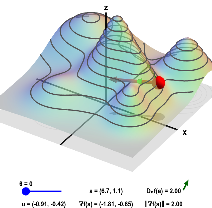
Geometric interpretation

The gradient has two linked meanings:

1. Direction: $\nabla f$ points in the direction of the steepest local increase in $f$.
2. Magnitude: $\Vert \nabla f\Vert$ is the largest possible local rate of increase per unit distance moved.

On a contour map, each contour joins points having the same function value. Moving along a contour does not change the function value, at least locally. Therefore, the gradient is perpendicular to the contour line and points across contours toward higher values.

The mountain image depicts this distinction. The gradient is the locally steepest uphill direction. A different direction can still go uphill, downhill, or stay level, but it generally changes the function less rapidly than the gradient direction.

The direction of steepest local decrease is

$$-\nabla f.$$

That negative gradient becomes important when training models: a loss is an error measure, so we normally seek a direction that decreases it rather than increases it.

Directional derivatives

A partial derivative measures change along one coordinate axis. But an input can move in any direction. For a unit direction vector $\mathbf{u}$, the directional derivative is

$$D_{\mathbf{u}}f=\nabla f(\mathbf{x}{)}^{\mathsf{T}}\mathbf{u}.$$

This is a dot product, connecting directly to the previous lesson.

The directional derivative answers:

If I move one unit in direction $\mathbf{u}$, what is the local rate of change in $f$?

Because it is a dot product:

• A positive value means that direction increases $f$.
• A negative value means that direction decreases $f$.
• A value of zero means the direction is locally level.
• The maximum possible value is $\Vert \nabla f\Vert$, achieved when $\mathbf{u}$ aligns with the gradient.
• The most negative value is $-\Vert \nabla f\Vert$, achieved when $\mathbf{u}$ points opposite the gradient.

This makes the gradient more than a list of coordinate-wise numbers. It is the object that predicts first-order change in every direction.

---

Why gradients matter in speech ML

In a speech-recognition system, a model might transform log-mel frames into token probabilities. During training, the model compares those predictions to the transcript and produces a scalar loss:

$$L(\mathbf{w}).$$

Here, $\mathbf{w}$ denotes all learned parameters: projection weights, convolution filters, attention matrices, normalization parameters, and more.

The gradient

$${\nabla }_{\mathbf{w}}L$$

answers a local sensitivity question for every parameter:

If this particular parameter increases slightly, how should the training loss change, with all other parameters held fixed?

A component with a positive gradient means increasing that parameter tends to increase loss locally. A component with a negative gradient means increasing it tends to reduce loss locally. The magnitude indicates how strongly the loss responds near the current parameter values.

For a model with a parameter matrix

$$\mathbf{W}\in {\mathbb{R}}^{80\times 256},$$

the loss gradient has matching shape:

$${\nabla }_{\mathbf{W}}L\in {\mathbb{R}}^{80\times 256}.$$

That shape is not incidental. It contains one sensitivity value for every learned weight connecting the 80 input features to the 256-dimensional representation.

In PyTorch, automatic differentiation will eventually compute these gradients. But software can only be used responsibly when its output has a clear interpretation: parameter.grad is not a mysterious set of numbers. It is a tensor of local loss sensitivities, aligned element-by-element with that parameter tensor.

---

Important cautions

Statement	Correct interpretation
“The derivative is the change in a function.”	It is the local rate of change, not the total finite change over a large interval.
“A zero gradient means the minimum has been found.”	Not necessarily. It can be a local minimum, local maximum, saddle point, or flat region.
“A partial derivative tells how the function changes when all inputs change.”	No. It changes one input while holding the rest fixed.
“The gradient is a scalar slope.”	For a scalar output with many inputs, it is a vector of sensitivities.
“The gradient points toward the best solution.”	It points toward steepest increase. For loss minimization, the negative gradient is the relevant local direction.

The word local is essential throughout. Gradients summarize behavior near the current point; they do not guarantee what will happen after a large parameter change or across a complicated nonconvex loss surface.

---

Key takeaways

• A derivative, $f^{\prime }(x)$ or $\frac{df}{dx}$, measures instantaneous local change of a one-input function.
• A partial derivative, such as $\frac{\partial f}{\partial x}$, measures local change with respect to one input while other inputs are fixed.
• The gradient, $\nabla f$, is a vector containing all partial derivatives of a scalar-valued function.
• The gradient points in the direction of steepest local increase, and its norm gives the largest local increase rate per unit distance.
• The negative gradient points toward steepest local decrease, which is why gradients underpin model training.
• For a scalar loss, the gradient has the same shape as the input parameter tensor it differentiates with respect to.

Next, you will move from interpretation to computation: calculating gradients of simple multivariable functions by applying ordinary derivative rules one variable at a time.