Neural Audio Codec Discretization

Hello! Welcome to the tenth module of our course.

In previous modules, we explored powerful Text-to-Speech systems like Tacotron 2 and VITS. A common theme was the use of an intermediate representation—the mel-spectrogram—from which a vocoder would generate the final audio waveform. We are now about to pivot to a new and exciting paradigm that is powering the latest generation of audio models: treating audio as a sequence of discrete tokens, much like words in a sentence.

This lesson directly addresses the learning outcome: Explain how neural audio codecs like SoundStream or EnCodec discretize audio waveforms into a sequence of tokens. Understanding this process is the key that unlocks the ability to apply powerful Language Model architectures, like the Transformer, directly to audio generation tasks.

Let's begin by understanding why we need to move beyond generating audio sample-by-sample.

1. The Challenge of Raw Audio

A raw audio waveform is a sequence of continuous values. A standard 16 kHz audio signal has 16,000 samples for every second of audio. If we wanted to generate audio by predicting one sample at a time, a model would need to make 160,000 predictions just to create a 10-second clip. This poses two major problems:

1. Extreme Sequence Length: Transformer models, while powerful, struggle with such long sequences. Their attention mechanism has a computational cost that scales quadratically with sequence length, making it infeasible to capture dependencies over more than a fraction of a second.
2. Slow Inference: Generating audio one sample at a time is incredibly slow, making real-time applications impossible.

To see why this approach is so challenging, let's turn to an excellent blog post that explores this exact problem.

As the article demonstrates, we need a way to compress the audio into a more manageable, shorter sequence of meaningful units. This is where neural audio codecs come in.

2. The Core Idea: Autoencoders and Vector Quantization

The general approach to solving this is to use an autoencoder, a type of neural network trained to compress an input into a low-dimensional latent representation and then reconstruct the original input from that representation.

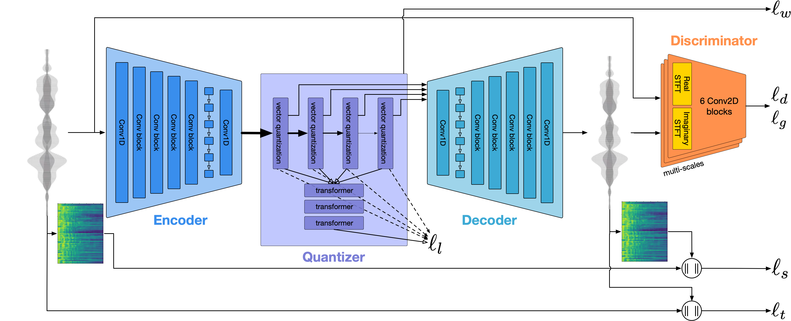
The key components are:

1. Encoder: A neural network (typically a 1D CNN) that takes the long raw audio waveform $x$ and maps it to a shorter sequence of continuous latent vectors $z$.
2. Decoder: A network that takes the latent vectors $z$ and reconstructs the audio waveform $\hat{x}$.

However, a standard autoencoder produces continuous latent vectors. For use with language models, we need discrete tokens. The solution is Vector Quantization (VQ).

VQ works by maintaining a codebook, which is essentially a list of embedding vectors (codewords). During the forward pass, each continuous vector produced by the encoder is replaced by the closest vector from the codebook. We then pass the index of that closest vector to the language model.

This process is a cornerstone of models like VQ-VAE (Vector-Quantized Variational Autoencoder). The next resource provides a fantastic and intuitive explanation of this concept.

3. Scaling Up with Residual Vector Quantization (RVQ)

Simple VQ has a major limitation. To achieve high reconstruction quality, we need to capture fine details, which would require a very large codebook (e.g., millions of entries). This is computationally expensive and memory-intensive.

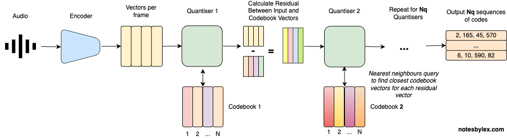
The solution is Residual Vector Quantization (RVQ). Instead of using one massive codebook, RVQ uses a series of smaller codebooks in a cascade.

The process is as follows:

1. The first quantizer finds the closest codeword in its codebook to the original embedding vector.
2. It then calculates the residual error: the difference between the original vector and the chosen codeword.
3. This residual error is passed to the second quantizer, which finds the closest codeword in its codebook to represent this error.
4. This process repeats for a set number of quantizers, with each stage quantizing the residual error from the previous stage.

The final discrete representation for the original vector is the set of indices from all the quantizers. This is like representing a precise location with a series of progressively finer details: country, then state, then city, then street address.

Let's dive into two resources that explain RVQ in detail.

The core benefit of RVQ is its efficiency. If you have $N_q$ quantizers, each with a codebook of size $C$, you can represent $C^{N_q}$ distinct values while only needing to store $N_q\times C$ codebook vectors. For example, 8 codebooks of size 1024 can represent over $10^{24}$ values, while only storing 8192 vectors.

4. Case Studies: SoundStream and EnCodec

Now that we understand the building blocks, let's see how they are assembled in two seminal neural audio codec models: Google's SoundStream and Meta's Encodec. Both models use a convolutional autoencoder with a Residual Vector Quantizer and are trained with a GAN-style adversarial loss to achieve high perceptual quality.

SoundStream

SoundStream introduced the end-to-end neural audio codec framework that combines a learned encoder/decoder with RVQ.

EnCodec

Encodec builds upon the principles of SoundStream but introduces several architectural improvements, including using a Transformer to speed up the quantization process during inference.

5. From Multi-level Codes to a Single Token Stream

The final step is to convert the output of the RVQ into a flat sequence of tokens that a language model can process. An RVQ with $N_q$ quantizers produces $N_q$ parallel streams of codes. For a language model, we need a single sequence.

The standard approach is to flatten these streams, typically in a time-first or quantizer-first manner. For example, for a given time step $t$, you would lay out the code from the first quantizer, then the second, and so on, before moving to time step $t+1$.

[code_t1_q1, code_t1_q2, ..., code_t1_qNq, code_t2_q1, code_t2_q2, ...]

This flattened sequence of integer indices is what is finally fed into a Transformer model, just like tokenized text.

---

Conclusion

In this lesson, we have demystified the process of audio discretization, a fundamental step for modern audio generation. You now understand how continuous, high-dimensional audio waveforms are transformed into discrete, manageable sequences of tokens.

Key Takeaways:

• The Problem: Modeling raw audio sample-by-sample is computationally infeasible due to extremely long sequence lengths.
• The Solution: Neural audio codecs use an autoencoder architecture to compress audio into a latent representation.
• Discretization: Vector Quantization (VQ) maps these continuous latent vectors to discrete indices from a learned codebook.
• Scalability: Residual Vector Quantization (RVQ) makes this process practical by using a cascade of smaller codebooks to quantize the residual error at each stage, achieving high fidelity with a manageable number of parameters. The error decreases exponentially for a linear increase in the number of codebooks.
• The Output: The codec produces several parallel streams of integer codes, which are then flattened into a single sequence of tokens, ready to be modeled by a language model.

Preview of the Next Lesson:

Now that we have our sequence of discrete audio tokens, what do we do with them? In the next lesson, we will describe how a standard language model architecture (e.g., a decoder-only Transformer) can be applied to discrete audio tokens for generation, looking at pioneering models like AudioLM. This is where we truly begin to treat audio as a new language.