Analyzing Time, Space, and Amortized Complexity in Java Solutions

Hello, and welcome to the first lesson in your interview-preparation course.

This first module rebuilds the coding-interview foundation needed for Staff and Principal-level backend interviews: not just producing a correct solution, but explaining why it scales, what it stores, and where its guarantees have limits. In this lesson, you will practice giving a precise complexity analysis of Java code, including the distinction between worst-case, expected, and amortized cost.

For interview purposes, a complexity statement is part of the solution, not an afterthought. A strong answer names the input variables, identifies the dominant work, states the relevant guarantee, and accounts for memory honestly.

---

Complexity is a growth-rate contract

Let $T(n)$ be the running time of a method on an input of size $n$. Asymptotic notation describes how $T(n)$ grows as inputs become large.

• $O(g(n))$ is an asymptotic upper bound.
• $\Omega (g(n))$ is an asymptotic lower bound.
• $\Theta (g(n))$ is a tight bound: both upper and lower.

In a coding interview, saying “time complexity is $O(n)$” usually means “the worst-case running time is linear in the number of input elements,” unless you explicitly state a different qualifier. Do not treat $O$ as automatically synonymous with worst case; it is an upper-bound notation. The qualifier matters particularly for hashing and dynamically resized collections.

A useful mental model is that Big-O intentionally ignores:

• Constant multipliers, such as $5n$.
• Lower-order terms, such as $n^2+20n+3$, which is $O(n^2)$.
• Machine-specific execution details.

It does not mean constants never matter. An allocation-heavy $O(n)$ Java implementation can be much slower than a cache-friendly $O(n)$ implementation. At interview scale, establish asymptotic correctness first; discuss practical overhead when it affects a design choice.

Start by defining the input size

Before analyzing code, declare what each variable represents.

• One array or string of length $n$: use $n$.
• Two independent arrays of lengths $n$ and $m$: use both $n$ and $m$.
• A matrix with $r$ rows and $c$ columns: use $r$ and $c$, giving $O(rc)$ for a full scan.
• Later, for graphs, the natural variables will be vertices $V$ and edges $E$.

Collapsing everything into $n$ can hide the actual cost. For example, comparing every element of one list with every element of another costs $O(nm)$, not necessarily $O(n^2)$.

A reliable way to count work

When reading a Java solution, apply this sequence:

1. Identify the dominant operations. Examples include comparisons, hash lookups, heap updates, array copies, or calls to a helper method.
2. Count how often each operation can occur.
3. Combine sequential phases by addition. Keep the dominant term asymptotically.
4. Multiply only for truly independent nested work.
5. State the guarantee: worst-case, expected, or amortized.
6. Analyze memory separately.

For sequential phases, costs add:

$$O(n)+O(n\log n)+O(n)=O(n\log n)$$

For a branch, the worst-case cost is the larger branch, not the sum of both branches:

$$\max (O(n),O(n\log n))=O(n\log n)$$

A loop that halves a search range each iteration is logarithmic:

$$O(\log n)$$

A loop that processes all $n$ elements at each of $\log n$ levels, such as merge sort, is:

$$O(n\log n)$$

---

Nested loops: inspect total movement, not indentation

One of the most common analysis mistakes is declaring every nested loop to be $O(n^2)$. That conclusion is correct only when the inner loop performs a full $O(n)$ traversal for each outer-loop iteration.

Consider this window-maintenance pattern:

static int longestWithinLimit(int[] values, int limit) {
    int left = 0;
    int sum = 0;
    int best = 0;

    for (int right = 0; right < values.length; right++) {
        sum += values[right];

        while (sum > limit) {
            sum -= values[left];
            left++;
        }

        best = Math.max(best, right - left + 1);
    }

    return best;
}

At first glance, the while loop is nested inside the for loop. But left never moves backward. Across the entire method:

• right advances at most $n$ times.
• left advances at most $n$ times.
• Each array element is added once and removed at most once.

The total pointer movement is bounded by $2n$, so the time complexity is:

$$O(n)$$

The method uses only a fixed number of primitive local variables:

$$O(1)$$

auxiliary space.

This accounting style will be essential in the next sliding-window lesson. The rule is not “nested loops are linear”; it is: prove a global bound on the inner loop’s total work.

By contrast, this loop does enumerate roughly every pair:

for (int i = 0; i < n; i++) {
    for (int j = i + 1; j < n; j++) {
        process(i, j);
    }
}

Its operation count is:

$$(n-1)+(n-2)+\cdots +1$$

which is:

$$\Theta (n^2)$$

---

Expected time: what hashing actually guarantees

Hash-based lookup is one of the most important interview tools, but its complexity must be described accurately.

static boolean containsDuplicate(int[] values) {
    Set<Integer> seen = new HashSet<>();

    for (int value : values) {
        if (!seen.add(value)) {
            return true;
        }
    }

    return false;
}

Let $n$ be values.length.

Under the usual assumption that hashes distribute keys well:

• HashSet.add is expected $O(1)$.
• The loop performs at most $n$ additions.
• Total expected time is $O(n)$.
• The set can store up to $n$ values, so auxiliary space is $O(n)$.

A high-quality interview explanation would be:

“Let $n$ be the number of array elements. I scan the array once and maintain a HashSet of values already seen. Each membership-and-insert operation is expected constant time under the normal hashing assumption, giving expected $O(n)$ time and $O(n)$ auxiliary space. The method can return earlier if it finds a duplicate, but the worst case scans the whole array.”

There are three different ideas here:

Guarantee	What varies?	Example
Worst-case	The input or structure state is unfavorable	Linear scan finds the target last
Expected	Cost is analyzed under a probability assumption	Hash lookup with well-distributed hashes
Amortized	Cost is spread across a sequence of operations	Repeated ArrayList.add operations

Expected time does not mean “it is fast most of the time” in an informal sense. It rests on an explicit probabilistic model, such as uniform hash distribution. Amortized time does not depend on randomness at all.

A related Java caveat: HashMap and HashSet may resize internally, and pathological collisions can affect observed behavior. In ordinary coding interviews, state the expected hashing assumption. In a production design discussion, also consider attacker-controlled keys, hashCode() quality, load factor, allocation pressure, and whether an ordered structure would provide more predictable behavior.

---

Space complexity: count memory deliberately

Space complexity needs its own statement. In interviews, the usual convention is to report auxiliary space: memory allocated beyond the input itself.

For containsDuplicate:

• Input array: $O(n)$, but normally excluded from auxiliary space.
• HashSet<Integer>: up to $O(n)$ entries.
• Local references and counters: $O(1)$.

Therefore:

$$\text{Auxiliary space}=O(n)$$

For the window example, there is no extra collection and no recursion:

$$\text{Auxiliary space}=O(1)$$

Use these distinctions consistently:

Memory source	Usually counted as auxiliary space?	Notes
Local primitives and references	Yes	Often $O(1)$
New arrays, maps, sets, queues	Yes	Count their maximum size
Recursion call stack	Yes	Depth matters
Input array or input string	No	State this convention if relevant
Returned output	Depends	State whether output space is included
In-place mutation of input	No extra structure	May still have stack space

For recursive Java methods, do not report only the heap allocations. If recursion reaches depth $n$, its call stack is $O(n)$, even if the method creates no collection.

Autoboxing changes practical memory usage: HashSet<Integer> stores boxed Integer objects rather than raw int values. That does not change the asymptotic result of $O(n)$, but it can matter in high-throughput services and memory-sensitive code.

---

Amortized analysis: expensive operations that happen rarely

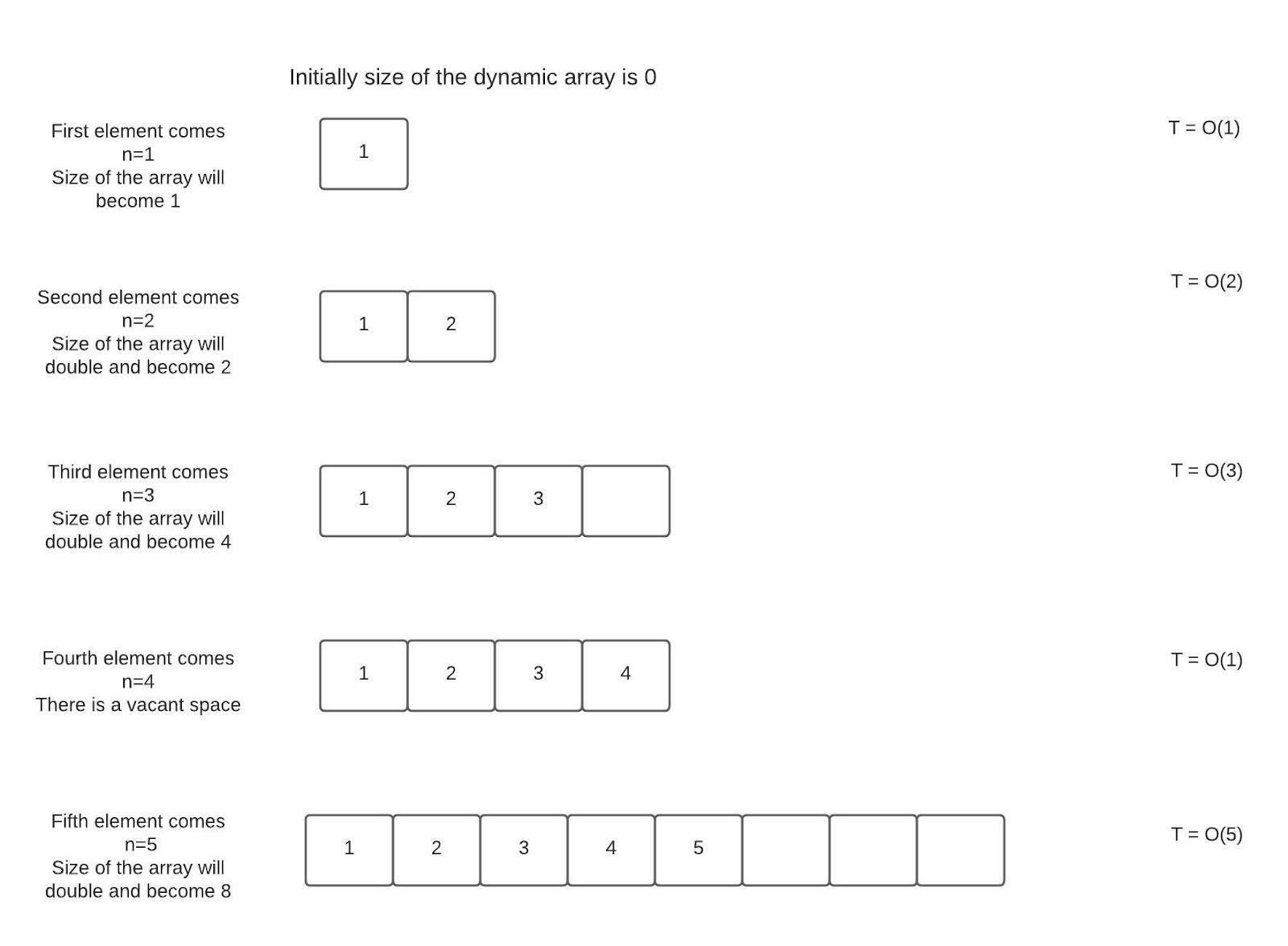
A dynamic array has an apparent contradiction:

• Adding an element to an array with spare capacity is $O(1)$.
• Adding an element when it is full may allocate a larger array and copy all existing elements, which is $O(n)$.

Java’s ArrayList is backed by a dynamically resized array. Its exact capacity-growth policy is an implementation detail, but the important property is geometric growth: capacity increases by a constant factor rather than by a fixed number of slots.

Suppose capacity begins at $1$ and doubles whenever it becomes full. Across $n$ append operations:

• The $n$ new elements must each be written once, costing $O(n)$.
• Resize copies occur at capacities $1,2,4,8,\dots$.

The total copying work is bounded by a geometric series:

$$1+2+4+\cdots +2^k<2n$$

So the work for all $n$ appends is bounded by:

$$T(n)<n+2n=3n$$

Therefore:

$$T(n)=O(n)$$

Dividing the total by the number of appends gives constant amortized cost per append:

$$\frac{T(n)}{n}=O(1)$$

The word amortized is crucial. It does not say every individual append is constant time. A specific append that triggers a resize remains $O(n)$. It says any long sequence of appends has a total cost linear in the number of appends.

Why fixed-size growth fails

Suppose an array increases capacity by only $100$ elements each time it fills.

To hold $n$ elements, it resizes roughly $n/100$ times. The copy costs resemble:

$$100+200+300+\cdots +n$$

This sum is quadratic:

$$\Theta (n^2)$$

The average cost per append is then $\Theta (n)$, not constant. The difference is structural:

• Geometric growth: larger copies occur much less often, giving amortized $O(1)$ append.
• Fixed-increment growth: increasingly large copies occur too frequently, giving non-constant amortized append.

The accounting intuition

One way to explain amortization informally is the accounting method. Charge every append three abstract units:

1. One unit pays for placing the new element.
2. The remaining units are saved as credit.
3. When a resize occurs, saved credit pays for copies.

The stored credit must never become negative. This establishes that a constant charge per append covers all actual work over the sequence.

For an interview, the aggregate proof is typically enough. In a more algorithmically rigorous setting, the potential method gives a state-based proof. If the array has $q$ stored elements and capacity $c$, one valid potential function for doubling is:

$$\Phi =2q-c$$

The amortized cost of an operation is:

$$\widehat{c_i}=c_i+\Phi (D_i)-\Phi (D_{i-1})$$

where $c_i$ is actual cost and $D_i$ is the structure after operation $i$. Regular appends accumulate potential; resizing spends it. Both kinds of appends have constant amortized cost.

You do not need to derive potential functions during a typical product-company coding interview. You should, however, be able to state precisely:

“ArrayList.add at the end is amortized $O(1)$, because occasional resize-and-copy operations have total linear cost across $n$ appends. A resize-triggering append itself is $O(n)$.”

Also distinguish it from insertion at an arbitrary position:

• arrayList.add(value) at the end: amortized $O(1)$.
• arrayList.add(index, value) in the middle: $O(n)$, because elements after index must shift.
• arrayList.get(index): $O(1)$.

---

An interview-ready complexity report

After writing a solution, use this compact reporting structure:

1. Define input variables.
   “Let $n$ be the number of values.”

2. Describe the traversal and dominant operations.
   “The loop visits each value once, and each lookup is expected constant time.”

3. State the correct time qualifier.
   “Expected $O(n)$ time because the implementation uses hashing.”
   Or: “Amortized $O(1)$ per append because the backing array grows geometrically.”

4. State auxiliary space and name the allocation.
   “The hash set stores at most $n$ values, so auxiliary space is $O(n)$.”

5. Mention relevant caveats only when useful.
   “A single resize can be linear, but the sequence cost is amortized constant.”
   “Hashing relies on normal distribution assumptions.”

For example, a concise answer for the duplicate-detection method is:

“Let $n$ be the array length. I make one pass through the input. The HashSet stores each distinct value once, so it uses $O(n)$ auxiliary space. Under the standard uniform-hashing assumption, add is expected $O(1)$, making total expected runtime $O(n)$.”

This is much stronger than simply saying “one loop, so $O(n)$.” It identifies the hidden data-structure operation, the guarantee being claimed, and the memory cost.

---

Key takeaways

• Complexity analysis begins by defining the real input variables, such as $n$, $m$, $r$, and $c$.
• Sum sequential phases, multiply independent nested traversals, and analyze total pointer movement before calling nested loops quadratic.
• Report expected time for hash-based operations when relying on normal hash distribution.
• Report auxiliary space separately from time, including collections and recursion stack.
• An ArrayList append can be $O(n)$ on a resize, yet repeated appends are amortized $O(1)$ because geometric resizing makes total copy work $O(n)$.
• In an interview, state assumptions and qualifiers rather than presenting a bare Big-O label.

Next, you will apply this discipline to a core coding pattern: using a hash-based lookup strategy to solve an array or string problem efficiently.