Kinematics of Particle Motion

Hello! Welcome to the first lesson in our module on Dynamics.

In our previous modules, we focused on Statics—the analysis of bodies at rest or moving with a constant velocity. We finished by learning how to predict if a component would fail under a given load. Now, we shift our focus to Dynamics, the study of bodies in accelerated motion. This is the bedrock of aerospace engineering, essential for analyzing everything from a rocket's launch trajectory to an aircraft's flight path.

This lesson begins our study of kinematics, which is the geometry of motion. We'll describe how things move (their position, velocity, and acceleration) without yet considering the forces that cause the motion. Specifically, this lesson addresses the learning outcome: Apply kinematic equations to solve problems of rectilinear and curvilinear motion for a particle.

We will start with motion in a straight line (rectilinear) and then extend those concepts to motion along a curved path (curvilinear) using a familiar x-y coordinate system.

1. Describing Motion: Position, Velocity, and Acceleration

Before we can solve problems, we need a common language to describe motion. Let's start with a particle moving in a straight line, a concept known as rectilinear motion.

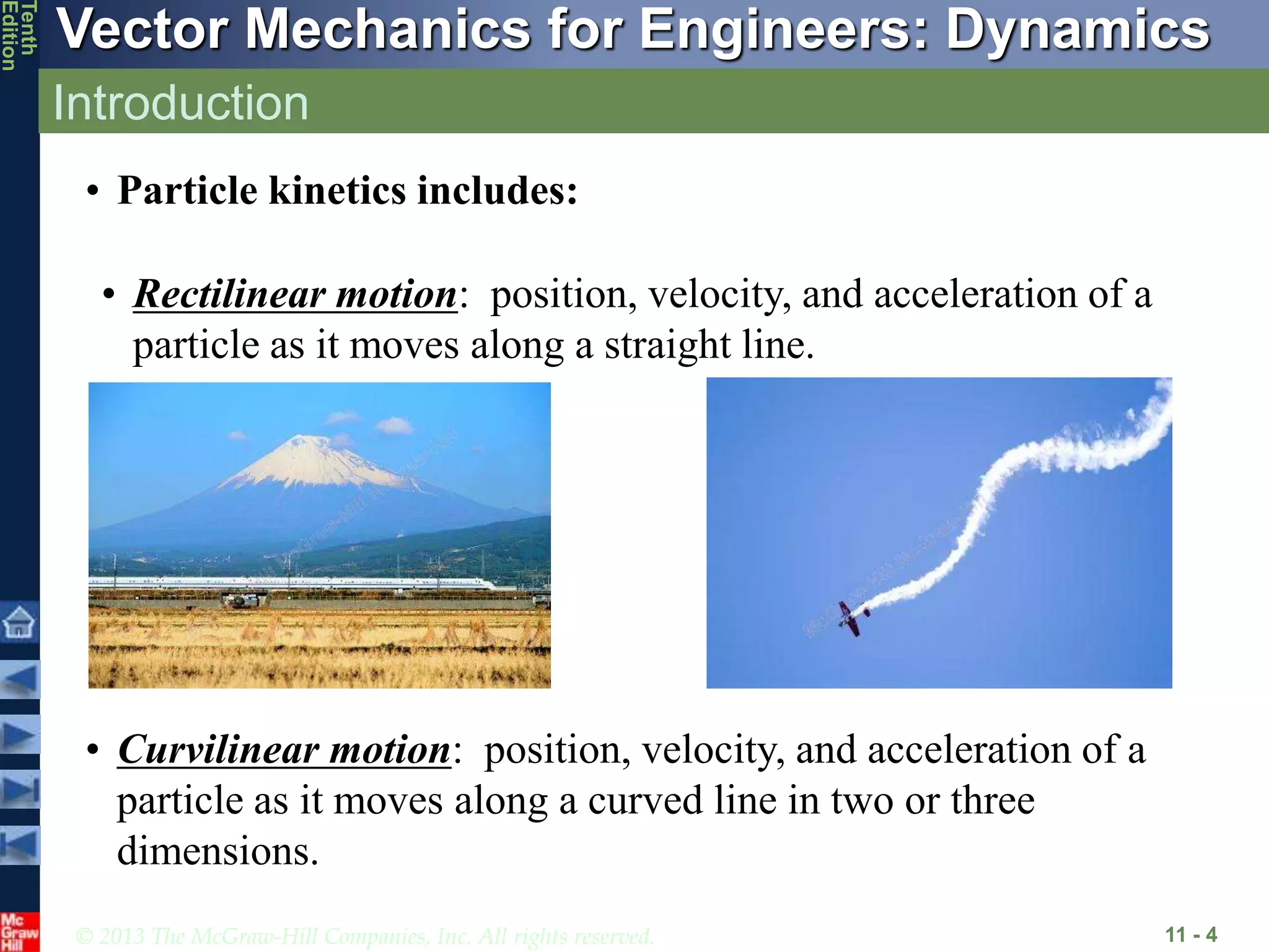
The fundamental quantities we use are:

• Position ($s$): The location of a particle relative to a fixed origin.
• Displacement ($\Delta s$): The change in position of a particle. It's a vector quantity, so direction matters.
• Velocity ($v$): The rate of change of position. It's also a vector. Its magnitude is called speed.
• Acceleration ($a$): The rate of change of velocity.

These quantities are linked by calculus. If position is a function of time, $s(t)$, then:

• Velocity: $v=\frac{ds}{dt}$
• Acceleration: $a=\frac{dv}{dt}=\frac{d^{2}s}{d{t}^2}$

Your background in electronics engineering has prepared you for this kind of analysis. These relationships are analogous to the fundamental differential equations in circuit theory, such as $i(t)=C\frac{dv(t)}{dt}$ for a capacitor. In both fields, calculus provides the language to describe how quantities change over time.

We can also find a useful relationship by eliminating time:

• From $v=ds/dt$, we get $dt=ds/v$.
• From $a=dv/dt$, we get $dt=dv/a$.
• Equating these gives $ds/v=dv/a$, which we rearrange into the powerful time-independent equation: $ads=vdv$.

2. Rectilinear Motion: Constant and Variable Acceleration

Most introductory problems in dynamics fall into two categories based on acceleration.

a) Constant Acceleration

This is a very common special case. A classic example is an object in free fall near the Earth's surface, where acceleration due to gravity, $g$, is approximately constant ($9.81{\text{m/s}}^2$ or $32.2{\text{ft/s}}^2$).

When acceleration $a_c$ is constant, we can integrate the fundamental differential equations to get three key algebraic formulas that you will use frequently.

1. Velocity as a function of time:
   $v=v_0+a_{c}t$
2. Position as a function of time:
   $s=s_0+v_{0}t+\frac{1}{2}{a}_c{t}^2$
3. Velocity as a function of position:
   $v^2=v_0^2+2a_c(s-s_0)$

Here, $s_0$ and $v_0$ are the initial position and velocity at $t=0$. These equations are the core toolkit for constant acceleration problems.

b) Variable Acceleration (Erratic Motion)

When acceleration is not constant but changes with time, position, or velocity (e.g., $a=2t$, $a=4s$, or $a=-0.4v^3$), we cannot use the simple constant acceleration formulas. Instead, we must go back to the fundamental differential equations and perform integration or differentiation.

This is often visualized using graphs of position, velocity, and acceleration versus time (s-t, v-t, a-t). The relationships are:

• The slope of the s-t graph is velocity.
• The slope of the v-t graph is acceleration.
• The area under the a-t graph is the change in velocity.
• The area under the v-t graph is the change in position (displacement).

Test your understanding!

A car starts from rest and accelerates according to the relation $a=6t+4$, where $a$ is in m/s² and $t$ is in seconds. What is its velocity after 4 seconds, and how far has it traveled?

Show answer

Since acceleration is a function of time, we must integrate.

1. Find velocity (v):
   We know $a=dv/dt$, so $dv=adt$.
   ${\int }_{v_0}^{v}dv={\int }_0^t(6t+4)dt$
   Since the car starts from rest, $v_0=0$.
   $v=[3t^2+4t{]}_0^t=3t^2+4t$
   At $t=4$ s:
   $v=3(4{)}^2+4(4)=3(16)+16=48+16=64\text{m/s}$

2. Find position (s):
   We know $v=ds/dt$, so $ds=vdt$.
   ${\int }_{s_0}^{s}ds={\int }_0^t(3t^2+4t)dt$
   Assuming it starts from the origin, $s_0=0$.
   $s=[t^3+2t^2{]}_0^t=t^3+2t^2$
   At $t=4$ s:
   $s=(4{)}^3+2(4{)}^2=64+2(16)=64+32=96\text{m}$

Answer: The velocity is 64 m/s and the distance traveled is 96 m.

3. Curvilinear Motion: Rectangular Components

When a particle moves along a curved path, its velocity and acceleration vectors change in both magnitude and direction. The simplest way to analyze this is to break the motion down into components using a fixed rectangular (Cartesian) coordinate system (x, y, z).

The vector equations for motion are:

• Position: $\vec{r}=x\hat{i}+y\hat{j}$
• Velocity: $\vec{v}=v_x\hat{i}+v_y\hat{j}$, where $v_x=\dot{x}$ and $v_y=\dot{y}$
• Acceleration: $\vec{a}=a_x\hat{i}+a_y\hat{j}$, where $a_x={\dot{v}}_x$ and $a_y={\dot{v}}_y$

The great advantage of this method is that the motion in each coordinate direction is treated as a separate rectilinear motion problem. All the equations we just learned for rectilinear motion apply independently to the x and y components.

Application: Projectile Motion

A crucial application for aerospace is projectile motion. This describes the motion of an object (a ball, a satellite, a ballistic missile) that is thrown or launched and then moves only under the influence of gravity.

By neglecting air resistance, we make two key assumptions:

1. The horizontal acceleration is zero: $a_x=0$.
2. The vertical acceleration is constant and directed downward: $a_y=-g$.

This simplifies the kinematics greatly:

Horizontal Motion ($a_x=0$)	Vertical Motion ($a_y=-g$)
$v_x=(v_0{)}_x$	$v_y=(v_0{)}_y-gt$
$x=x_0+(v_0{)}_{x}t$	$y=y_0+(v_0{)}_{y}t-\frac{1}{2}g{t}^2$
	$v_y^2=(v_0{)}_y^2-2g(y-y_0)$

These three equations (one for x, two for y) allow you to solve for any three unknown quantities in a projectile motion problem (e.g., time of flight, maximum height, range).

Conclusion

In this lesson, you've taken the first step into dynamics by learning the principles of kinematics. You now have a solid, formula-based toolkit to describe and solve problems involving particle motion.

Key Takeaways:

• Kinematics describes motion using position, velocity, and acceleration, which are linked by differentiation and integration.
• Rectilinear motion is motion in a straight line. If acceleration is constant, a set of three simple algebraic equations can be used. If it's variable, you must use calculus.
• Curvilinear motion is motion along a curved path. Using rectangular coordinates, we can break the motion into independent rectilinear problems for each axis.
• Projectile motion is a key application of curvilinear motion where horizontal velocity is constant ($a_x=0$) and vertical acceleration is constant ($a_y=-g$).

Next Lesson Preview:

Using rectangular coordinates is powerful, but it's not always the most convenient method, especially for objects that are rotating or following a circular path. In our next lesson, we will explore a different way to analyze curvilinear motion by looking at motion in normal and tangential coordinates. This will give us a more direct way to understand how an object's speed and direction are changing along its curved path.