First-Order Trotter-Suzuki for Hamiltonian Simulation

Hello! Welcome back to our deep dive into quantum computing.

In our previous lessons, we focused on the Variational Quantum Eigensolver (VQE), a hybrid algorithm designed to find the static ground state energy of a Hamiltonian. We saw how to construct the necessary components and implement the full workflow for the H₂ molecule.

Today, we shift our focus from static properties to the dynamics of quantum systems. This lesson addresses the learning outcome: Implement Hamiltonian simulation using a first-order Trotter-Suzuki decomposition and analyze its gate complexity and error scaling. We will explore how to simulate the time evolution of a quantum state, a task for which quantum computers are believed to hold a significant advantage over classical ones.

1. The Challenge of Simulating Quantum Dynamics

The evolution of a closed quantum system over time $t$ is described by the Schrödinger equation, whose solution is given by the application of a unitary operator $U(t)=e^{-iHt}$ to an initial state $|\psi (0)⟩$, where $H$ is the system's Hamiltonian (we set $\hslash =1$).

The core task of Hamiltonian simulation is to implement this unitary operator $U(t)$ on a quantum computer.

If the Hamiltonian $H$ can be implemented as a single quantum gate, this is trivial. However, most Hamiltonians of interest, like those you encountered in VQE, are sums of many simple terms:

$$H=\sum _{k=1}^{\Gamma }{H}_k$$

For example, in the transverse-field Ising model, the terms are local Pauli operators like $Z_i{Z}_{i+1}$ and $X_i$. While we can easily implement the evolution for each individual term $e^{-i{H}_{k}t}$, we cannot simply multiply them together to get the total evolution. This is because, in general, the terms do not commute ($[H_j,H_k]\ne 0$), and for non-commuting operators $A$ and $B$, the identity $e^{A+B}=e^A{e}^B$ fails.

This is the central problem that Hamiltonian simulation algorithms must solve. The most direct approach is called Trotterization or Trotter-Suzuki decomposition.

2. The First-Order Trotter-Suzuki Decomposition

The foundation of Trotterization is the Lie-Trotter product formula, which states that for operators $A$ and $B$:

$$e^{A+B}=\underset{N\to \infty }{\lim }(e^{A/N}{e}^{B/N}{)}^N$$

This formula becomes an approximation when we use a large but finite number of steps, $N$. For a small time step $\delta t$, the first-order Trotter-Suzuki formula gives us a practical approximation:

$$e^{-iH\delta t}=e^{-i({\sum }_k{H}_k)\delta t}\approx \prod _k{e}^{-i{H}_k\delta t}+O(\delta t^2)$$

The error in this approximation for a single step is of the order $\delta t^2$.

To simulate the evolution for a total time $t$, we break the evolution into $N$ small, discrete time steps of duration $\delta t=t/N$. We then apply the first-order approximation for each step.

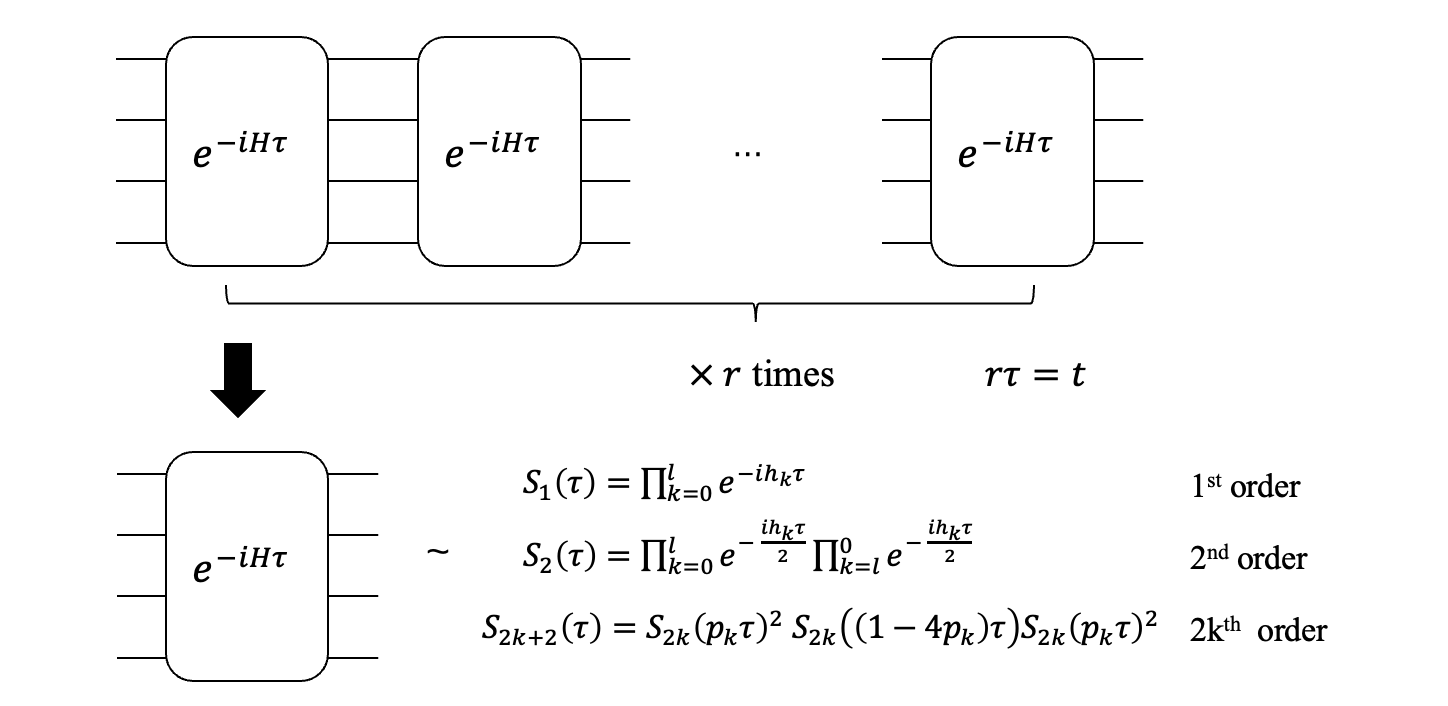
The full evolution is thus approximated by:

$$U(t)=e^{-iHt}\approx {\left(\prod _{k=1}^{\Gamma }{e}^{-i{H}_k(t/N)}\right)}^N$$

This decomposes the complex, large-scale evolution into a sequence of simpler unitaries that we can implement with basic quantum gates.

3. Error Analysis and Gate Complexity

Understanding the performance of an algorithm requires analyzing its resource costs (gate complexity) and its accuracy (error scaling).

Error Scaling

As we saw, the error of a single Trotter step of size $\delta t=t/N$ is $O(\delta t^2)=O((t/N{)}^2)$. When we concatenate $N$ such steps, the errors add up. A common heuristic suggests the total error $ϵ$ scales as:

$$ϵ\approx N\times O\left({\left(\frac{t}{N}\right)}^2\right)=O\left(\frac{t^2}{N}\right)$$

This crucial result tells us that to achieve a desired accuracy $ϵ$, the number of Trotter steps $N$ must be proportional to $t^2/ϵ$. The error decreases as we increase $N$, as you'll see demonstrated in the video later.

For a more rigorous understanding, which your background supports, the error bound depends on the structure of the Hamiltonian. For $H=A+B$, the error of a single first-order step is bounded by:

$$\Vert e^{-it(A+B)}-e^{-itB}{e}^{-itA}\Vert \le \frac{t^2}{2}\Vert [A,B]\Vert$$

This shows that the approximation error is directly related to how much the Hamiltonian terms fail to commute.

Gate Complexity

The gate complexity is the total number of elementary gates required for the simulation. Let's estimate it for a Hamiltonian $H={\sum }_{k=1}^{\Gamma }{H}_k$.

1. Cost per Trotter step: To implement one step, we must implement $\Gamma$ unitaries of the form $e^{-i{H}_k(t/N)}$. Let's say the gate cost for the $k$-th term is $C_k$. The total cost for one step is roughly ${\sum }_{k=1}^{\Gamma }{C}_k$.
2. Number of steps: To achieve a target error $ϵ$, we need $N=O(t^2/ϵ)$ steps.
3. Total Gate Complexity: Combining these, the total complexity is: $$\text{Total Cost}=N\times \left(\sum _{k=1}^{\Gamma }{C}_k\right)=O\left(\frac{t^2}{ϵ}\sum _{k=1}^{\Gamma }{C}_k\right)$$

This analysis reveals how the simulation cost scales with the evolution time $t$, the desired precision $ϵ$, and the complexity of the Hamiltonian itself (both the number of terms $\Gamma$ and the cost to implement them $C_k$).

4. Implementation: The Transverse-Field Ising Model

Let's make this concrete by implementing a simulation for the transverse-field Ising model, a cornerstone model in quantum magnetism. Its Hamiltonian on $n$ qubits is:

$$H=J\sum _{i=0}^{n-2}{Z}_i{Z}_{i+1}+h\sum _{i=0}^{n-1}{X}_i$$

This Hamiltonian is an excellent test case because the interaction terms ($Z_i{Z}_{i+1}$) do not commute with the transverse-field terms ($X_i$), making Trotterization necessary.

To build the circuit for one Trotter step of duration $\delta t$, we need to sequence the circuits for each term:

$$U_{\text{step}}(\delta t)\approx \left(\prod _{i=0}^{n-2}{e}^{-iJ\delta t{Z}_i{Z}_{i+1}}\right)\left(\prod _{i=0}^{n-1}{e}^{-ih\delta t{X}_i}\right)$$

• Transverse-field terms: The evolution $e^{-ih\delta t{X}_i}$ is simply a rotation around the X-axis, implemented by an RX gate: $R_X(2h\delta t)$.
• Interaction terms: The two-qubit term $e^{-iJ\delta t{Z}_i{Z}_{i+1}}$ can be decomposed using CNOT and RZ gates. The identity is: $$e^{-i\theta Z_i{Z}_{i+1}}={\text{CNOT}}_{i,i+1}(I\otimes R_Z(2\theta )){\text{CNOT}}_{i,i+1}$$ This works because conjugating a single-qubit $Z$ rotation on the target qubit by a CNOT gate effectively turns it into a two-qubit $ZZ$ rotation.

The comparison with the exact solution in the tutorial is a practical demonstration of the error analysis we discussed. By changing the number of steps M in the code, you can directly observe how the approximation improves as M increases, just as our $O(t^2/N)$ scaling predicted.

To reinforce this, let's see a visual example of this convergence.

Conclusion

In this lesson, we have explored the fundamentals of simulating quantum dynamics on a digital quantum computer. We moved from the static problem of finding ground states to the dynamic problem of simulating time evolution.

Key Takeaways:

• Hamiltonian simulation aims to implement the time evolution operator $U(t)=e^{-iHt}$.
• When a Hamiltonian $H$ is a sum of non-commuting terms, we cannot simply multiply the individual evolution operators.
• The first-order Trotter-Suzuki decomposition provides a practical solution by approximating the evolution over a small time step $\delta t$: $e^{-iH\delta t}\approx {\prod }_k{e}^{-i{H}_k\delta t}$.
• The total evolution for time $t$ is simulated by repeating this approximation for $N$ steps, where $\delta t=t/N$.
• The error of this method scales as $O(t^2/N)$, meaning the number of steps must grow quadratically with time and inversely with the desired precision.
• The gate complexity scales as $O(\frac{t^2}{ϵ}\Gamma \bar{C})$, where $\Gamma$ is the number of Hamiltonian terms and $\bar{C}$ is their average implementation cost.
• We saw how to implement this for the transverse-field Ising model by decomposing each term's evolution into a sequence of elementary quantum gates.

Preview of the Next Lesson

The technique of simulating evolution under a Hamiltonian is a powerful building block. In our next lesson, Construct the QAOA ansatz circuit for a given problem Hamiltonian, such as for MaxCut, we will see how this idea is repurposed for optimization problems. The Quantum Approximate Optimization Algorithm (QAOA) uses an ansatz that alternates between evolution under a "problem" Hamiltonian and a "mixer" Hamiltonian. The evolution times become the variational parameters, creating a powerful link between Hamiltonian simulation and the variational algorithms we studied earlier.