Equations of Motion for Rigid Bodies in General Planar Motion

Hello! In our last lesson, we established how to calculate the mass moment of inertia, $I$, which is a body's resistance to angular acceleration. We are now ready to put that concept to use.

Today, we will learn how to apply the three equations of motion for a rigid body in general planar motion. This is the heart of rigid body kinetics. We are moving from describing motion (kinematics) to explaining the causes of motion (kinetics). These equations are the direct equivalent of Newton's Second Law ($F=ma$) but expanded to handle bodies that both translate and rotate simultaneously, a common scenario for aerospace components like landing gear, control surfaces, or even a satellite deploying its solar arrays.

1. The Three Fundamental Equations of Motion

General planar motion is a combination of the translation of the body's center of mass and the rotation of the body about its center of mass. Consequently, we need a set of equations that governs both aspects.

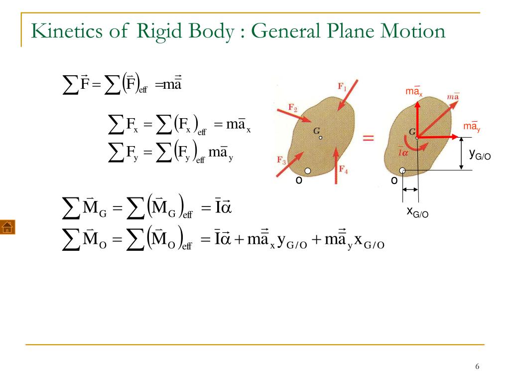
For any rigid body in planar motion, we have three fundamental equations:

1. Sum of forces in the x-direction: $\sum F_x=m{a}_{Gx}$
2. Sum of forces in the y-direction: $\sum F_y=m{a}_{Gy}$
3. Sum of moments about the center of mass (G): $\sum M_G=I_G\alpha$

Here:

• $\sum F_x$ and $\sum F_y$ are the sums of all external forces acting on the body.
• $m$ is the mass of the body.
• $a_{Gx}$ and $a_{Gy}$ are the x and y components of the linear acceleration of the body's center of mass, G.
• $\sum M_G$ is the sum of all external moments (torques) about the center of mass, G.
• $I_G$ is the mass moment of inertia about the center of mass, which you learned to calculate in the last lesson.
• $\alpha$ is the angular acceleration of the body.

To visualize this, engineers often use two diagrams side-by-side:

• A Free-Body Diagram (FBD), which you know well, showing all external forces and moments.
• A Kinetic Diagram, which shows the result of these forces: the linear acceleration vector $m{\vec{a}}_G$ and the angular acceleration term $I_G\vec{\alpha }$.

The equations of motion simply state that the FBD is equivalent to the Kinetic Diagram.

2. A General Problem-Solving Strategy

Solving problems in rigid body kinetics requires a systematic approach. The following four-step method is highly effective:

1. Diagrams: Draw a Free-Body Diagram (FBD) showing all external forces (weight, normal forces, friction, applied forces). Then, draw a Kinetic Diagram showing the $m{\vec{a}}_G$ and $I_G\alpha$ terms. Establish a coordinate system.
2. Kinetics Equations: Apply the three equations of motion based on your diagrams.
3. Kinematics: Often, the three kinetics equations will have more than three unknowns. You must find additional equations by analyzing the geometry of motion (kinematics). A classic example is the no-slip condition for a rolling object.
4. Solve: Count your equations and unknowns. Once you have a sufficient number of equations, solve the system algebraically.

3. Application: Rolling Motion and the No-Slip Condition

A very common and important case of general planar motion is an object rolling on a surface. This is relevant to aircraft wheels during takeoff and landing.

If an object rolls without slipping, there is a direct relationship between its linear and angular acceleration. This provides the crucial kinematic equation we often need. For a wheel of radius $r$, this condition is:
$a_G=\alpha r$

However, rolling is possible due to friction. If the required friction force to prevent slipping is greater than the maximum available static friction ($f_{max}={\mu }_{s}N$), the object will slip. This is a critical check you must perform.

The following video works through an excellent example of a wheel with an applied moment. Pay close attention to the process:

1. Assume the wheel rolls without slipping and use $a_G=\alpha r$.
2. Solve for the unknowns, including the friction force $f$.
3. Check if the friction force required is possible: Is $f\le {\mu }_{s}N$?
4. If the condition is violated, the initial assumption was wrong. You must re-solve the problem using the kinetic friction force, $f={\mu }_{k}N$, and in this case, $a_G$ and $\alpha$ are independent unknowns ($a_G\ne \alpha r$).

4. An Alternative: Summing Moments About Other Points

While summing moments about the center of mass G ($\sum M_G=I_G\alpha$) always works, it's not always the most efficient method. Sometimes, choosing a different point can eliminate unknown forces and simplify the algebra.

A particularly powerful shortcut is to sum moments about the Instantaneous Center of Zero Velocity (IC). For an object rolling without slipping, the IC is the point of contact with the ground. The moment equation becomes simpler:
$\sum M_{IC}=I_{IC}\alpha$
Notice two things:

1. The forces acting at the IC (normal force and friction) produce no moment about the IC, so they disappear from the equation.
2. You must use the moment of inertia about the IC, $I_{IC}$. You can find this using the parallel axis theorem you learned last lesson: $I_{IC}=I_G+m{d}^2$, where $d$ is the distance from G to the IC (which is the radius, $r$, for a rolling wheel).

Let's see how this shortcut works in practice.

Test your understanding!

A uniform solid cylinder of mass $m=10$ kg and radius $r=0.2$ m is placed on a 30° incline. The coefficient of static friction is ${\mu }_s=0.4$. The cylinder is released from rest. Determine the acceleration of its center of mass, $a_G$, and the friction force, $f$. (For a solid cylinder, $I_G=\frac{1}{2}m{r}^2$).

Hint: Assume it rolls without slipping, solve for $a_G$ and $f$, and then check if the friction assumption is valid.

Show answer

1. Diagrams and Equations:

• FBD: Forces are weight ($mg$) acting vertically down, normal force ($N$) perpendicular to the incline, and friction ($f$) acting up the incline (opposing the tendency to slide down).
• Coordinate System: Let the x-axis be parallel to the incline, pointing down, and the y-axis be perpendicular to the incline, pointing up.
• The weight component parallel to the incline is $mg\sin (30^{\circ })$.
• The weight component perpendicular to the incline is $mg\cos (30^{\circ })$.

2. Kinetics Equations:

• $\sum F_y=N-mg\cos (30^{\circ })=0⟹N=(10)(9.81)\cos (30^{\circ })=84.96$ N.
• $\sum F_x=mg\sin (30^{\circ })-f=m{a}_G⟹(10)(9.81)\sin (30^{\circ })-f=10a_G⟹49.05-f=10a_G$. (Eq. 1)
• $\sum M_G=f\cdot r=I_G\alpha$. (Eq. 2)

We have two equations but three unknowns ($f,a_G,\alpha$). We need a kinematic relation.

3. Kinematics (Assume No-Slip):

• Assume rolling without slipping: $a_G=\alpha r$, so $\alpha =a_G/r=a_G/0.2$.
• Substitute $I_G=\frac{1}{2}m{r}^2=\frac{1}{2}(10)(0.2{)}^2=0.2$ kg·m².
• Substitute into Eq. 2: $f\cdot (0.2)=(0.2)\cdot (a_G/0.2)⟹0.2f=a_G$. (Eq. 3)

4. Solve:

• Now we have two equations for $f$ and $a_G$. Substitute Eq. 3 into Eq. 1:
  $49.05-f=10(0.2f)⟹49.05-f=2f⟹3f=49.05⟹f=16.35$ N.
• Now find $a_G$ using Eq. 3: $a_G=0.2(16.35)=3.27$ m/s².

5. Check the Friction Assumption:

• The friction force required to prevent slipping is $f=16.35$ N.
• The maximum available static friction is $f_{max}={\mu }_{s}N=0.4\cdot (84.96)=33.98$ N.
• Since $f<f_{max}$ ($16.35\text{ N}<33.98\text{ N}$), our assumption was correct. The cylinder rolls without slipping.

Final Answer:

• The acceleration is $a_G=3.27$ m/s².
• The friction force is $f=16.35$ N.

Conclusion

Today you've learned the cornerstone of rigid body kinetics: how to relate the forces on an object to the motion it experiences. This is a huge step towards analyzing complex mechanical and aerospace systems.

Key Takeaways:

• General planar motion is governed by three equations: $\sum F_x=m{a}_{Gx}$, $\sum F_y=m{a}_{Gy}$, and $\sum M_G=I_G\alpha$.
• Solving kinetics problems is a systematic process involving FBDs, kinetic equations, and kinematic relationships.
• For rolling without slipping, the kinematic constraint $a_G=\alpha r$ is essential, but you must always verify the friction assumption ($f\le {\mu }_{s}N$).
• Summing moments about the Instantaneous Center (IC) can be a powerful shortcut, especially in rolling problems.

Next Lesson Preview:
In the next lesson, we will focus on a special case of general planar motion: fixed-axis rotation. This occurs when a body is pinned about an axis that does not move, like a turbine rotor or a hinged control surface. We will see how today's equations simplify for this common and important scenario.