Computing Gradients with Respect to Vector Parameters

Welcome back. In the previous lesson, we wrote a linear model for a dataset as

$$\hat{\mathbf{y}}=\mathbf{X}\mathbf{\beta }$$

with rows representing observations and columns representing features. That notation now gives us a precise answer to a practical training question: if the model’s total error changes, which parameter should change, and by how much?

This lesson develops the mathematical object that answers it: the gradient of a scalar loss with respect to a vector of parameters. You will compute gradients from partial derivatives, derive the gradient for squared-error linear regression, and interpret the resulting vector in a way that makes the next lesson’s gradient-descent update rule almost inevitable.

---

A scalar loss, many adjustable parameters

To focus on training rather than prediction notation, write the model parameters as

$$\mathbf{w}=\left[\begin{array}{c}{w}_0\\ w_1\\ ⋮\\ w_p\end{array}\right]$$

The intercept may be included as $w_0$, paired with a constant feature $x_0=1$, exactly as in the prior lesson. A model fitted to data has one scalar objective value:

$$L(\mathbf{w})\in \mathbb{R}$$

The loss $L$ is a single number: for example, total squared prediction error, average log loss, or that loss plus a regularization penalty. But it depends on every entry of $\mathbf{w}$.

For a scalar function of vector parameters, the gradient collects one partial derivative per parameter:

$${\nabla }_{\mathbf{w}}L(\mathbf{w})=\left[\begin{array}{c}\frac{\partial L}{\partial w_0}\\ \frac{\partial L}{\partial w_1}\\ ⋮\\ \frac{\partial L}{\partial w_p}\end{array}\right]$$

We will use the convention that gradients are column vectors, so the gradient has the same shape as its parameter vector. Each component says how rapidly the loss changes when only that parameter is varied and all other parameters are held fixed.

For example, consider the simple loss

$$L(w_1,w_2)=3w_1^2+2w_1{w}_2-w_2$$

Its two partial derivatives are

$$\frac{\partial L}{\partial w_1}=6w_1+2w_2$$ $$\frac{\partial L}{\partial w_2}=2w_1-1$$

Therefore,

$${\nabla }_{\mathbf{w}}L=\left[\begin{array}{c}6w_1+2w_2\\ 2w_1-1\end{array}\right]$$

At $\mathbf{w}=[1,2{]}^{\top }$, the gradient is

$${\nabla }_{\mathbf{w}}L=\left[\begin{array}{c}10\\ 1\end{array}\right]$$

A small positive change in $w_1$ raises the loss much more strongly than an equally sized positive change in $w_2$, locally at that point.

The gradient is not just a bundle of derivatives. For a small parameter displacement $\Delta \mathbf{w}$,

$$L(\mathbf{w}+\Delta \mathbf{w})\approx L(\mathbf{w})+{\nabla }_{\mathbf{w}}L(\mathbf{w}{)}^{\top }\Delta \mathbf{w}$$

This first-order approximation says that the gradient identifies the direction of greatest local increase in loss. Consequently, its negative identifies the direction of greatest local decrease for a fixed, sufficiently small displacement. We will turn that observation into gradient descent in the next lesson.

---

A small derivative toolkit

Most conventional ML objectives can be decomposed into a small number of patterns. When in doubt, expand an expression into components and differentiate one parameter at a time; compact matrix identities are conveniences, not substitutes for reasoning.

Scalar function of $\mathbf{w}$	Gradient with respect to $\mathbf{w}$	Why
$c$, a constant	$0$	No parameter affects a constant.
${\mathbf{a}}^{\top }\mathbf{w}$	$\mathbf{a}$	Each $w_j$ occurs as $a_j{w}_j$.
$\frac{1}{2}\Vert \mathbf{w}{\Vert }_2^2$	$\mathbf{w}$	This is $\frac{1}{2}{\sum }_j{w}_j^2$.
${\mathbf{w}}^{\top }\mathbf{Aw}$	$(\mathbf{A}+{\mathbf{A}}^{\top })\mathbf{w}$	A parameter can occur in both positions of the quadratic form.
$\frac{1}{2}{\mathbf{w}}^{\top }\mathbf{Aw}$, with $\mathbf{A}$ symmetric	$\mathbf{Aw}$	Symmetry makes the two contributions equal.

The most reusable rule is the gradient of a dot product:

$${\nabla }_{\mathbf{w}}\left({\mathbf{a}}^{\top }\mathbf{w}\right)=\mathbf{a}$$

It is the vector version of the one-variable rule that the derivative of $aw$ with respect to $w$ is $a$.

This immediately gives a compact chain-rule pattern. If

$$L(\mathbf{w})=g({\mathbf{a}}^{\top }\mathbf{w})$$

where $g$ is any differentiable scalar function, then

$${\nabla }_{\mathbf{w}}L=g^{\prime }({\mathbf{a}}^{\top }\mathbf{w})\mathbf{a}$$

The scalar factor $g^{\prime }({\mathbf{a}}^{\top }\mathbf{w})$ measures the sensitivity of the outer loss; the vector $\mathbf{a}$ distributes that sensitivity across the parameters.

A practical caveat: sources differ on whether they write a derivative with respect to a vector as a row or a column. This is a notation convention, sometimes called numerator versus denominator layout. Rather than memorizing formula sheets blindly, establish the convention at the start and check dimensions throughout. In this lesson,

$${\nabla }_{\mathbf{w}}L\in {\mathbb{R}}^{(p+1)\times 1}$$

because

$$\mathbf{w}\in {\mathbb{R}}^{(p+1)\times 1}$$

---

Deriving the squared-error gradient for one observation

Consider one observation $({\mathbf{x}}_i,y_i)$. The linear model score is

$$z_i={\mathbf{x}}_i^{\top }\mathbf{w}$$

and, for regression, the score itself is the prediction:

$${\hat{y}}_i=z_i$$

Use a half-squared-error loss for this one observation:

$${\ell }_i(\mathbf{w})=\frac{1}{2}{\left({\mathbf{x}}_i^{\top }\mathbf{w}-y_i\right)}^2$$

The factor $\frac{1}{2}$ does not change which parameter values minimize the loss. It simply cancels the factor of $2$ produced when differentiating the square.

Introduce the residual

$$r_i={\hat{y}}_i-y_i={\mathbf{x}}_i^{\top }\mathbf{w}-y_i$$

Then

$${\ell }_i(\mathbf{w})=\frac{1}{2}{r}_i^2$$

To derive the gradient without relying on a remembered identity, take the partial derivative with respect to one parameter $w_j$:

$$\frac{\partial {\ell }_i}{\partial w_j}=\frac{\partial {\ell }_i}{\partial r_i}\frac{\partial r_i}{\partial w_j}$$

The outer derivative is

$$\frac{\partial {\ell }_i}{\partial r_i}=r_i$$

For the inner derivative, expand the score:

$$r_i=x_{i0}{w}_0+x_{i1}{w}_1+\cdots +x_{ip}{w}_p-y_i$$

Only the term $x_{ij}{w}_j$ depends on $w_j$, so

$$\frac{\partial r_i}{\partial w_j}=x_{ij}$$

Combining the two pieces gives

$$\frac{\partial {\ell }_i}{\partial w_j}=r_i{x}_{ij}$$

Stacking these component derivatives produces the gradient:

$${\nabla }_{\mathbf{w}}{\ell }_i=r_i{\mathbf{x}}_i=\left({\mathbf{x}}_i^{\top }\mathbf{w}-y_i\right){\mathbf{x}}_i$$

This formula deserves interpretation. An observation contributes a gradient proportional to:

1. Its signed residual: underprediction produces a negative residual; overprediction produces a positive residual.
2. Its feature vector: parameters associated with large feature values receive a larger contribution.

If the prediction is exactly correct, $r_i=0$, that observation contributes a zero gradient. If a feature is zero for this observation, its corresponding coefficient receives no direct gradient contribution from that observation.

---

From one observation to a dataset

For $n$ observations, stack feature vectors into the design matrix $\mathbf{X}$, and stack targets into $\mathbf{y}$:

$$\mathbf{X}\in {\mathbb{R}}^{n\times (p+1)}$$ $$\mathbf{w}\in {\mathbb{R}}^{(p+1)\times 1}$$ $$\mathbf{y}\in {\mathbb{R}}^{n\times 1}$$

The vector of predictions and residuals is

$$\hat{\mathbf{y}}=\mathbf{Xw}$$ $$\mathbf{r}=\mathbf{Xw}-\mathbf{y}$$

Define the average half-squared-error loss:

$$J(\mathbf{w})=\frac{1}{2n}{\Vert \mathbf{Xw}-\mathbf{y}\Vert }_2^2$$

The norm notation is shorthand for a sum of squared residuals:

$$J(\mathbf{w})=\frac{1}{2n}\sum _{i=1}^n{\left({\mathbf{x}}_i^{\top }\mathbf{w}-y_i\right)}^2$$

Since differentiation distributes over a sum, average the individual gradients:

$${\nabla }_{\mathbf{w}}J=\frac{1}{n}\sum _{i=1}^n{r}_i{\mathbf{x}}_i$$

The equivalent matrix expression is

$$\boxed{{\nabla }_{\mathbf{w}}J=\frac{1}{n}{\mathbf{X}}^{\top }\left(\mathbf{Xw}-\mathbf{y}\right)}$$

The transpose is essential. The residual vector has one entry per row of $\mathbf{X}$, whereas the gradient must have one entry per column, or feature:

$${\mathbf{X}}^{\top }\left(\mathbf{Xw}-\mathbf{y}\right):((p+1)\times n)(n\times 1)=(p+1)\times 1$$

The expression ${\mathbf{X}}^{\top }\mathbf{r}$ is a vector of feature–residual alignments. A coefficient’s gradient is large when its feature values tend to coincide with large residuals of one sign. At a least-squares optimum, these alignments balance out:

$${\mathbf{X}}^{\top }\mathbf{r}=0$$

That condition will later lead to the ordinary least-squares solution.

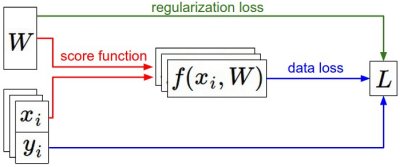
The data-flow diagram makes a useful modeling distinction. The data loss depends on predictions and labels. A regularization loss depends directly on the parameters and expresses a preference for simpler parameter values. The total loss is still a single scalar, so its gradient is simply the sum of the two gradient contributions.

For ridge-style $L_2$ regularization, the objective is

$$J_{\lambda }(\mathbf{w})=\frac{1}{2n}{\Vert \mathbf{Xw}-\mathbf{y}\Vert }_2^2+\frac{\lambda }{2}{\Vert \mathbf{w}\Vert }_2^2$$

Its gradient is

$${\nabla }_{\mathbf{w}}{J}_{\lambda }=\frac{1}{n}{\mathbf{X}}^{\top }\left(\mathbf{Xw}-\mathbf{y}\right)+\lambda \mathbf{w}$$

The $\lambda \mathbf{w}$ term increases with coefficient magnitude. In many libraries, the intercept is excluded from regularization; mathematically, this means applying the penalty only to the selected non-intercept entries rather than to every component of $\mathbf{w}$.

---

A complete numerical calculation

Take a model with an intercept and one feature:

$$\mathbf{X}=\left[\begin{array}{cc}1& 2\\ 1& 4\end{array}\right],\mathbf{y}=\left[\begin{array}{c}5\\ 8\end{array}\right],\mathbf{w}=\left[\begin{array}{c}1\\ 1\end{array}\right]$$

The predictions are

$$\mathbf{Xw}=\left[\begin{array}{c}3\\ 5\end{array}\right]$$

and the residuals are

$$\mathbf{r}=\mathbf{Xw}-\mathbf{y}=\left[\begin{array}{c}-2\\ -3\end{array}\right]$$

The average half-squared-error loss is

$$J(\mathbf{w})=\frac{1}{4}\left((-2{)}^2+(-3{)}^2\right)=3.25$$

Now compute the gradient:

$${\nabla }_{\mathbf{w}}J=\frac{1}{2}{\mathbf{X}}^{\top }\mathbf{r}$$ $$=\frac{1}{2}\left[\begin{array}{cc}1& 1\\ 2& 4\end{array}\right]\left[\begin{array}{c}-2\\ -3\end{array}\right]$$ $$=\frac{1}{2}\left[\begin{array}{c}-5\\ -16\end{array}\right]=\left[\begin{array}{c}-2.5\\ -8\end{array}\right]$$

Both entries are negative. Locally, increasing either parameter would decrease this particular loss; the feature coefficient has the larger magnitude because the larger feature values coincide with substantial underprediction.

The calculation also demonstrates why units and scaling matter. If the feature column were recorded in individual users rather than thousands of users, its values would be $1000$ times larger. The corresponding coefficient would need a different numerical scale, and its gradient would also have a dramatically different scale. The underlying predictions can be equivalent, but optimization behavior is not. We will examine that consequence directly in the next lesson.

---

Checking a gradient in code

Analytical gradients are fast and exact up to floating-point arithmetic. When implementing a nontrivial custom objective, a finite-difference gradient check is a valuable debugging tool.

For coordinate $w_j$, let ${\mathbf{e}}_j$ be the vector with a $1$ at position $j$ and zeros elsewhere. The central-difference estimate is

$$\frac{\partial J}{\partial w_j}\approx \frac{J(\mathbf{w}+ϵ{\mathbf{e}}_j)-J(\mathbf{w}-ϵ{\mathbf{e}}_j)}{2ϵ}$$

For a small fixed dataset, compare this approximation with the $j$-th entry of your analytical gradient:

import numpy as np

X = np.array([[1.0, 2.0],
              [1.0, 4.0]])
y = np.array([5.0, 8.0])
w = np.array([1.0, 1.0])

def mse_half(w, X, y):
    residuals = X @ w - y
    return 0.5 * np.mean(residuals ** 2)

def grad_mse_half(w, X, y):
    residuals = X @ w - y
    return X.T @ residuals / len(y)

analytic = grad_mse_half(w, X, y)

epsilon = 1e-6
numeric = np.zeros_like(w)

for j in range(len(w)):
    direction = np.zeros_like(w)
    direction[j] = 1.0
    numeric[j] = (
        mse_half(w + epsilon * direction, X, y)
        - mse_half(w - epsilon * direction, X, y)
    ) / (2 * epsilon)

print(analytic)
print(numeric)

The two vectors should be very close, though not character-for-character identical because the finite-difference expression itself is an approximation. If they disagree substantially, common causes include a missing averaging factor, an incorrect transpose, a sign error in the residual definition, or evaluating the loss and gradient on different data slices.

---

A gradient is the vector of partial derivatives of a scalar objective with respect to its parameter vector:

$${\nabla }_{\mathbf{w}}L=\left[\begin{array}{c}\frac{\partial L}{\partial w_0}\\ ⋮\\ \frac{\partial L}{\partial w_p}\end{array}\right]$$

For linear regression with average half-squared error, the central result is

$${\nabla }_{\mathbf{w}}J=\frac{1}{n}{\mathbf{X}}^{\top }\left(\mathbf{Xw}-\mathbf{y}\right)$$

It aggregates each observation’s residual, weighted by its feature values. Adding $L_2$ regularization contributes the additional gradient term $\lambda \mathbf{w}$.

Next, we will use the negative gradient to perform a gradient-descent update, then examine why learning rate and feature scale determine whether optimization converges smoothly, crawls, or diverges.