Understanding Sampling and Aliasing

Welcome to your second lesson.

In our first lesson, we established that a continuous sound wave can be modeled by the equation $y(t)=A\sin (2\pi ft+\varphi )$, where its properties of loudness, pitch, and timbre are captured by a combination of sinusoids. This represents the sound in its original, analog form.

However, your computer and the entire field of digital audio processing operate on discrete data, not continuous waves. The fundamental challenge is how to convert the continuous analog signal into a series of numbers—a process called sampling—without losing the information that makes up the sound.

This lesson focuses on the cornerstone principle that makes digital audio possible: the Nyquist-Shannon Sampling Theorem. We will explore what the theorem states, derive its formula by examining the process in the frequency domain, and demonstrate the critical distortion effect known as aliasing that occurs when the theorem's rules are broken.

1. From Continuous Waves to Discrete Samples

The process of converting a continuous signal to a discrete one is called sampling. It involves measuring the amplitude of the analog wave at regular, discrete intervals of time.

• The time between consecutive samples is the sampling period, denoted by $T_s$.
• The number of samples taken per second is the sampling rate (or sampling frequency), denoted by $f_s$, where $f_s=1/T_s$.

Imagine you have the smooth, continuous curve of an analog audio wave. Sampling is like laying a grid over it and recording the value of the curve only at each vertical line. The big question is: how close do those grid lines need to be to ensure you can perfectly redraw the original curve just from those recorded points?

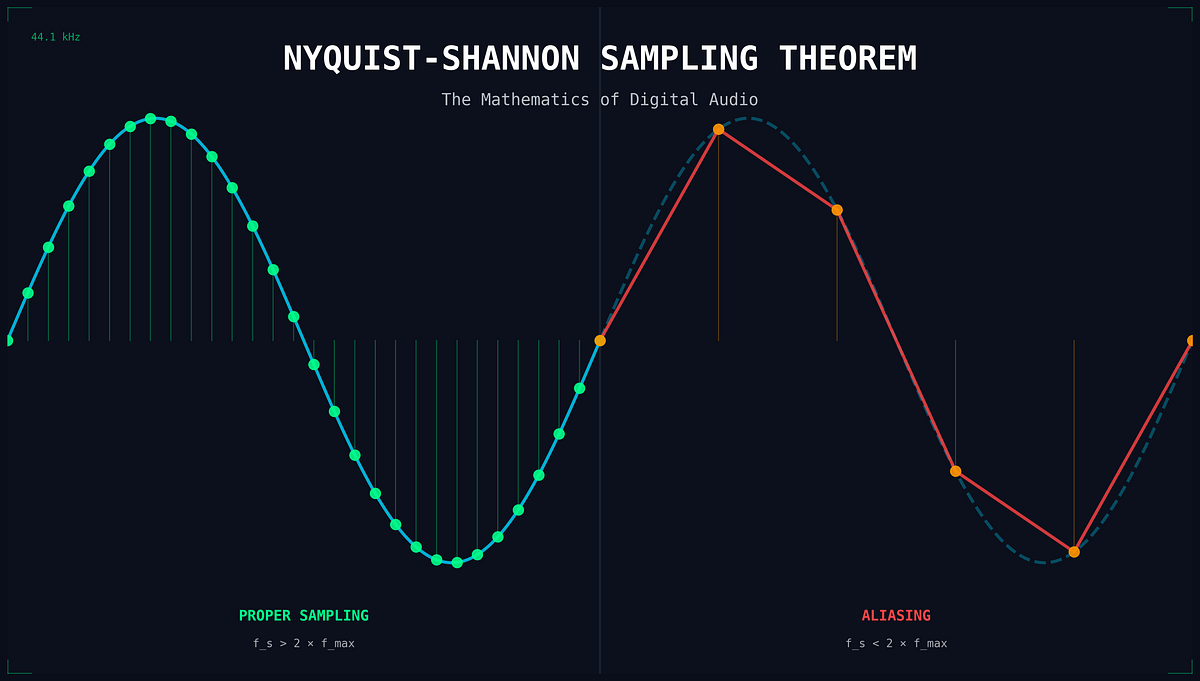
It might seem intuitive that you'll always lose some information between the samples. The astonishing conclusion of the Nyquist-Shannon theorem is that this is not true. Under a specific condition, you can capture all the information and achieve perfect reconstruction.

Let's begin with a high-level, intuitive explanation of this remarkable theorem.

2. The Nyquist-Shannon Sampling Theorem

As you just saw, the theorem provides the condition for this perfect reconstruction. Let's state it formally.

A signal is band-limited if its frequency content is confined to a finite range. For example, the range of human hearing is approximately 20 Hz to 20,000 Hz. Any audio signal intended for humans can be considered band-limited to this range.

The Nyquist-Shannon Sampling Theorem states:

If a continuous-time signal $x(t)$ contains no frequencies higher than $f_{max}$, it is completely determined by its samples if the sampling rate $f_s$ is greater than twice the maximum frequency.

$$f_s>2\cdot f_{max}$$

Let's clarify the terminology:

• $f_{max}$: The maximum frequency component in the signal.
• Nyquist Rate: The minimum sampling rate required for perfect reconstruction, which is exactly $2\cdot f_{max}$. The theorem states we must sample strictly greater than this rate, though in practice the term is often used for the boundary.
• Nyquist Frequency: Half of the sampling rate ($f_s/2$). This represents the maximum signal frequency that can be faithfully captured at a given sampling rate $f_s$. Any signal frequency above the Nyquist frequency will cause distortion.

3. Deriving the Theorem: A Frequency-Domain View

The "twice the highest frequency" rule can seem arbitrary at first. The proof and true understanding come from analyzing the effects of sampling in the frequency domain, which you'll find is a recurring and powerful technique in audio AI.

Given your background in CSE, you are familiar with the duality between time and frequency representations from concepts like the Fourier Transform. This is central to the derivation.

The following video provides a rigorous but clear walkthrough of the derivation. We will step through its key points.

Let's summarize the mathematical steps from the video:

1. Time Domain: Sampling a continuous signal $x(t)$ at intervals of $T_s$ can be modeled as multiplying $x(t)$ by an "impulse train" $p(t)$, which is a series of Dirac delta functions spaced $T_s$ apart. The resulting sampled signal is $x_p(t)=x(t)\cdot p(t)$.

2. Frequency Domain: The Convolution Theorem states that multiplication in the time domain corresponds to convolution in the frequency domain. We denote the Fourier Transforms of our signals with capital letters (e.g., $X(j\Omega )$). So, $X_p(j\Omega )=X(j\Omega )\ast P(j\Omega )$.

3. Spectrum of an Impulse Train: The Fourier Transform of an impulse train in time is another impulse train in frequency. The impulses in the frequency domain are spaced by the sampling frequency, ${\Omega }_s=2\pi f_s$.

4. Convolution: Convolving the original signal's spectrum, $X(j\Omega )$, with this frequency-domain impulse train creates periodic, shifted copies of $X(j\Omega )$ at every multiple of ${\Omega }_s$.

5. The Condition: If the original signal is band-limited to $\pm {\Omega }_{max}$, the copies of its spectrum will not overlap as long as the shift amount, ${\Omega }_s$, is greater than the width of the spectrum, $2{\Omega }_{max}$.

   $${\Omega }_s>2{\Omega }_{max}⟹2\pi f_s>2(2\pi f_{max})⟹f_s>2f_{max}$$

When this condition is met, we can perfectly recover the original spectrum (and thus the original signal) by using an ideal low-pass filter to cut off all the copies and keep only the central one.

Why $2\cdot f_{max}$? The Role of Negative Frequencies

You might wonder why the bandwidth is $2\cdot f_{max}$ and not just $f_{max}$. This is because for any real-valued signal (like audio), the frequency spectrum is symmetric around 0 Hz. If a 1000 Hz component exists, its "negative frequency" counterpart at -1000 Hz must also exist for the math to work out. The signal's energy is spread from $-f_{max}$ to $+f_{max}$, giving it a total bandwidth of $2\cdot f_{max}$.

For a formal text explanation, please read the following sections.

4. Aliasing: When Sampling Goes Wrong

Now we know the rule. But what happens if we break it? This is where we encounter aliasing.

If $f_s<2f_{max}$, the periodic copies of the spectrum overlap. This overlap is a form of corruption that is irreversible. In the overlapping regions, the high-frequency components from one copy get added to the low-frequency components of the next, and vice-versa. The result is that high frequencies are "folded" back into the lower frequency range, masquerading as frequencies that weren't in the original signal.

This phenomenon of a high frequency appearing as a lower one due to undersampling is called aliasing.

The aliased frequency, $f_{alias}$, can be calculated. For a signal frequency $f_{orig}$ that is above the Nyquist frequency ($f_s/2$), it will appear as a frequency reflected around $f_s/2$. A common case is:

For example, in a system with $f_s=44.1$ kHz, the Nyquist frequency is 22.05 kHz. A signal at 25 kHz is above this limit. It will alias and appear as a tone at $44.1-25=19.1$ kHz.

Once this happens, the 19.1 kHz alias is indistinguishable from a legitimate 19.1 kHz tone. The original information is lost forever.

To prevent aliasing, real-world analog-to-digital converters (ADCs) use a steep analog anti-aliasing filter before the sampling stage. This low-pass filter simply removes any frequencies above the Nyquist frequency ($f_s/2$), ensuring that the sampling condition is met.

5. Practical Demonstration with Python

Let's make this tangible. The following Python code uses numpy and matplotlib to simulate the sampling process and explicitly create aliasing.

import numpy as np
import matplotlib.pyplot as plt

def demonstrate_sampling(original_freq, sample_rate, duration=0.01):
    """
    Visualizes the effect of sampling a sine wave and shows aliasing.
    """



    # 1. Create a high-resolution 'analog' signal for reference
    analog_rate = 100 * original_freq  # High resolution for a smooth plot
    t_analog = np.linspace(0, duration, int(analog_rate * duration))
    analog_signal = np.sin(2 * np.pi * original_freq * t_analog)




    # 2. Sample the signal at the specified sample_rate
    num_samples = int(sample_rate * duration)
    t_digital = np.linspace(0, duration, num_samples)
    digital_samples = np.sin(2 * np.pi * original_freq * t_digital)




    # 3. Check for aliasing
    nyquist_freq = sample_rate / 2
    is_aliased = original_freq > nyquist_freq




    # 4. Plotting
    plt.figure(figsize=(12, 6))
    plt.plot(t_analog, analog_signal, label=f'Original Signal ({original_freq} Hz)', alpha=0.5)
    plt.stem(t_digital, digital_samples, linefmt='r-', markerfmt='ro', basefmt=' ', label=f'Sampled Points ({sample_rate} Hz)')

    if is_aliased:
        alias_freq = abs(sample_rate - original_freq)



        # Plot the aliased wave that the samples represent
        aliased_signal = np.sin(2 * np.pi * alias_freq * t_analog)
        plt.plot(t_analog, aliased_signal, 'g--', label=f'Aliased Signal ({alias_freq:.0f} Hz)')
        plt.title(f"ALIASING! {original_freq} Hz signal sampled at {sample_rate} Hz appears as {alias_freq:.0f} Hz", color='red')
    else:
        plt.title(f"Proper Sampling: {original_freq} Hz signal at {sample_rate} Hz")
    
    plt.xlabel("Time (s)")
    plt.ylabel("Amplitude")
    plt.legend()
    plt.grid(True)
    plt.show()




# --- Experiment Here ---




# Case 1: Proper Sampling
# Sampling a 1000 Hz signal at 20000 Hz (f_s > 2 * f_max)
demonstrate_sampling(original_freq=1000, sample_rate=20000)




# Case 2: Aliasing
# Sampling a 9000 Hz signal at 10000 Hz (f_s < 2 * f_max)
# Nyquist frequency is 5000 Hz. 9000 Hz should alias to 10000 - 9000 = 1000 Hz.
demonstrate_sampling(original_freq=9000, sample_rate=10000)

I encourage you to run this code and experiment with different values for original_freq and sample_rate. See if you can predict the alias frequency before you run the code for the second case. This will solidify the connection between the theory and its practical effect.

Conclusion

In this lesson, we bridged the gap between the continuous analog world and the discrete digital world. You now understand the fundamental law that governs this conversion.

Key Takeaways:

• Sampling is the process of converting a continuous signal into a discrete sequence of numbers by measuring its amplitude at regular intervals.
• The Nyquist-Shannon Sampling Theorem states that a band-limited signal can be perfectly reconstructed if the sampling rate $f_s$ is greater than twice its maximum frequency component $f_{max}$.
• The proof lies in the frequency domain: sampling in time creates periodic copies of the signal's spectrum in frequency. If $f_s>2f_{max}$, these copies do not overlap.
• Aliasing occurs when $f_s<2f_{max}$. The spectral copies overlap, causing high frequencies to "fold" into the lower frequency range, creating irreversible distortion.
• Anti-aliasing filters are used in practice to remove frequencies above the Nyquist limit before sampling to prevent aliasing.

You've now learned how a continuous wave is measured at discrete points in time. But what about the values of those measurements? The amplitudes are also continuous, and they too must be made discrete. This next step is called quantization.

In our next lesson, we will explore the process of quantization and how the bit depth of a digital audio file determines its dynamic range and fidelity.