Leak-Free Alignment and Resampling of Financial Time Series

Hello. You have already audited market data and transformed approved adjusted prices into simple and log returns. The next challenge is more subtle: a multi-asset dataset can look tidy while quietly mixing different trading calendars, stale values, and information that was not available at the time of a decision.

This lesson develops a defensible approach to aligning and resampling financial time series. You will learn to distinguish a missing observation from a zero return, construct multi-asset panels deliberately, aggregate data to lower frequencies with the right financial meaning, and use only information available at each decision time. These habits are essential for later portfolio optimization, volatility modeling, and credible backtests.

---

Alignment is a modeling decision, not a formatting step

Suppose you have adjusted daily prices for RELIANCE, INFY, and the NIFTY 50 index. Their timestamps may differ because of holidays, listing dates, data outages, or vendor coverage. A price matrix with dates as rows and assets as columns is convenient:

Date	RELIANCE	INFY	NIFTY 50
2024-01-02	2,580.40	1,450.20	21,665.80
2024-01-03	2,612.10	missing	21,517.35
2024-01-04	2,590.30	1,462.90	21,658.60

But the missing INFY value on 3 January has no universal meaning. It could indicate:

• a genuine exchange closure relevant to that instrument;
• a vendor outage;
• an incomplete data download;
• an asset that did not yet trade;
• a timestamp-conversion problem.

Replacing it automatically with the next day’s price is clearly invalid: that uses future information. Replacing it with the preceding price is sometimes appropriate for a valuation convention—for example, carrying a known prior close over a documented market holiday—but it is not automatically appropriate for computing observed returns or training a predictive model.

The central principle is:

At timestamp $t$, every value used by a model or trading rule must have been available no later than $t$.

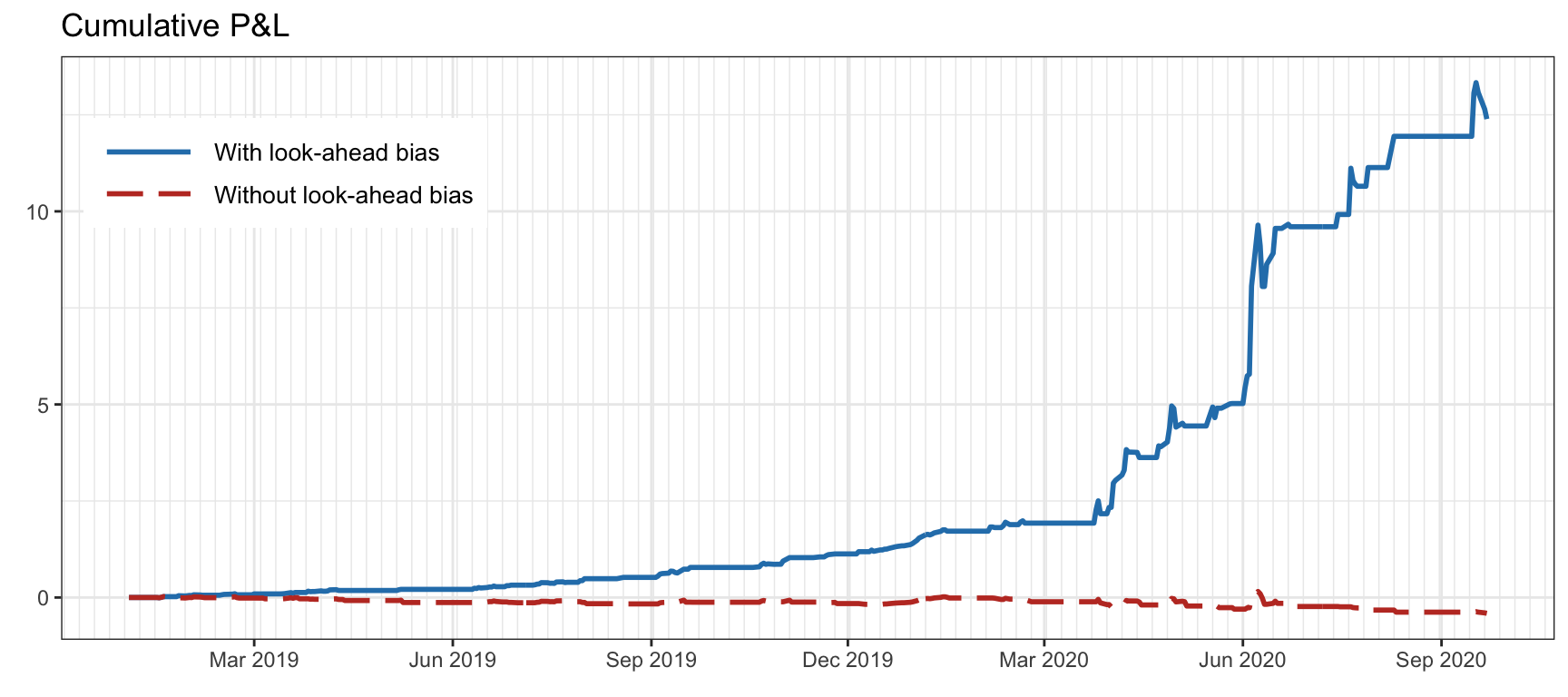
For trading research, this needs one further refinement. A daily closing price for 31 January is generally known only at, or after, the market close on 31 January. A strategy that acts at that same close cannot honestly use it unless its execution and data-arrival assumptions explicitly make that possible. The usual conservative convention is:

1. Compute a signal from information through the close of day $t$.
2. Form the position for day $t+1$.
3. Earn the return during day $t+1$.

In notation, if $s_t$ is a signal estimated with information available at $t$, then a daily strategy return is typically:

$$R_{p,t+1}=w_t{R}_{t+1}$$

where $w_t$ is the position chosen from $s_t$. The one-period shift between decision and realized return is not a minor coding detail; it is the boundary between a feasible strategy and look-ahead bias.

---

Put time semantics into the dataset

Before pivoting or resampling, make the time fields explicit. For daily end-of-day data, date may be enough if all instruments trade in the same market and you clearly define the close convention. For global assets, intraday data, macroeconomic releases, or quote data, use full timezone-aware timestamps.

A useful minimal long-format schema is:

timestamp,symbol,adj_close,source_timestamp
2024-01-02 15:30:00+05:30,RELIANCE,2580.40,2024-01-02 15:31:15+05:30
2024-01-02 15:30:00+05:30,INFY,1450.20,2024-01-02 15:31:15+05:30

The two timestamps serve different purposes:

• timestamp: when the market observation refers to;
• source_timestamp: when your data source made the observation available to your system.

For daily data obtained after the close, you may not know the exact vendor-arrival time. In that case, document a conservative assumption, such as “all day-$t$ closing data become usable at the next session’s open.” This assumption is more important than a false impression of timestamp precision.

Start by enforcing proper datetime types, uniqueness, and chronological order:

import pandas as pd


def validate_prices(prices: pd.DataFrame) -> pd.DataFrame:
    required = {"date", "symbol", "adj_close"}
    missing = required.difference(prices.columns)

    if missing:
        raise ValueError(f"Missing columns: {sorted(missing)}")

    data = prices.copy()
    data["date"] = pd.to_datetime(data["date"], errors="coerce")
    data["adj_close"] = pd.to_numeric(data["adj_close"], errors="coerce")

    if data["date"].isna().any():
        raise ValueError("Some dates could not be parsed.")

    if data.duplicated(["symbol", "date"]).any():
        duplicates = data.loc[
            data.duplicated(["symbol", "date"], keep=False),
            ["symbol", "date"]
        ]
        raise ValueError(
            "Duplicate symbol-date observations remain:\n"
            f"{duplicates.head()}"
        )

    return data.sort_values(["symbol", "date"]).reset_index(drop=True)

Do not “solve” duplicate observations with drop_duplicates() unless you have first identified the cause and chosen a documented resolution rule. A duplicate might be an accidental repeated row, an unadjusted and adjusted record mixed together, or two records from different exchanges.

---

Build a panel deliberately: union, intersection, and retained gaps

Once observations are valid, you can pivot the long table into a price panel:

prices = validate_prices(prices)

wide_prices = (
    prices.pivot(index="date", columns="symbol", values="adj_close")
          .sort_index()
)

print(wide_prices.head())

By default, this creates the union calendar: every date observed for at least one symbol appears. Missing values remain missing, which is usually the correct first output.

The next choice depends on the calculation.

Complete-case alignment

For a contemporaneous cross-sectional calculation—such as estimating a covariance matrix from daily returns—you may require all assets to have an observation on the same date:

complete_prices = wide_prices.dropna(how="any")

This gives an intersection calendar. It is transparent, but it can discard many rows when the asset universe is broad or spans markets with different holidays.

For example, a NIFTY constituent portfolio may be suited to a common NSE trading calendar. A panel combining NIFTY equities with US ETFs and European rates is more complicated: an intersection could unnecessarily remove valid observations from one market whenever another market is closed.

Keep the union and let missingness remain visible

For descriptive work or asset-specific return calculations, retain the union calendar:

coverage = wide_prices.notna().mean().sort_values()
print(coverage)

This reports the fraction of panel dates covered by each series. It is a useful diagnostic before choosing an estimation method. An asset with 70% coverage should not silently be treated as equivalent to one with 100% coverage.

A concise rule is:

Task	Common alignment choice
Inspect data quality and coverage	Union calendar; preserve missing values
Daily cross-sectional signal across a fixed universe	Complete cases or a documented eligibility rule
Portfolio valuation on a known non-trading day	Potentially carry prior price, with a stale-price flag
Return modeling for each asset	Compute returns per asset first; preserve gaps
International multi-market analysis	Use timestamps and a documented common decision time

Crucially, do not fill a missing return with zero. A zero return means the price was observed and unchanged. A missing return means you do not have enough valid information to establish the return.

---

Why prices and returns must be handled differently

The prior lesson established that returns are changes between valid prices. This distinction matters during alignment.

Consider a price observed on Friday and then again on Monday. Carrying Friday’s known closing price across Saturday and Sunday can make sense if you are creating a daily valuation grid. There was no weekend trading, so the prior close remains the last observable valuation.

However, creating artificial weekend returns of zero and then including them in volatility estimation is usually inappropriate. It dilutes the estimated variance simply by adding non-trading calendar days.

A safer sequence for daily research is:

1. Validate and sort each instrument’s adjusted-price history.
2. Calculate returns within each instrument’s observed trading sequence.
3. Pivot the resulting returns into a panel.
4. Decide how to treat dates with incomplete coverage for the specific analysis.

For a long-format return dataset from the previous lesson:

returns_long = (
    prices.sort_values(["symbol", "date"])
          .assign(
              simple_return=lambda x: (
                  x.groupby("symbol")["adj_close"]
                   .pct_change(fill_method=None)
              )
          )
)

return_panel = (
    returns_long.pivot(
        index="date",
        columns="symbol",
        values="simple_return",
    )
    .sort_index()
)

complete_return_panel = return_panel.dropna(how="any")

The fill_method=None makes the no-filling choice explicit. A gap remains a gap rather than being bridged by a carried-forward observation.

There is one limitation to notice. If a source omits an expected trading session entirely, the next valid return can span several sessions. That may be valid for an asset that genuinely did not trade, but it is often a data-quality concern for a liquid NIFTY 50 stock. Use the expected exchange calendar and the data audit from the earlier lesson to distinguish those cases. Do not let the calculation conceal them.

---

Resampling: choose an aggregation that matches the variable

Resampling changes frequency: daily observations to monthly observations, minute bars to daily bars, or daily data to a denser time grid. The correct method depends on what the column represents.

For price data, common downsampling rules are:

Variable	Weekly or monthly aggregation	Reason
Adjusted closing price	Last valid observation	Period-end valuation
Open price	First observation	First tradable value in period
High	Maximum	Period’s highest recorded price
Low	Minimum	Period’s lowest recorded price
Volume	Sum	Total activity over the period
Simple return	Compound gross returns	Preserves investment arithmetic
Log return	Sum	Preserves time additivity

Taking the monthly mean of closing prices may be useful for a descriptive chart, but it is not a month-end investable price and should not be used to calculate a conventional monthly return.

This short video gives a practical introduction to converting a dated series to a lower frequency. Its examples use straightforward aggregations; apply the financial interpretation above when selecting the aggregation function.

Monthly returns from prices

For reporting realized monthly returns, resample a valid daily price series to month-end observations and then calculate the percentage change:

monthly_prices = wide_prices.resample("ME").last()
monthly_returns = monthly_prices.pct_change(fill_method=None)

The return labeled 31 March is the realized return from the final available February price to the final available March price:

$$R_{\text{Mar}}=\frac{P_{\text{end of Mar}}}{P_{\text{end of Feb}}}-1$$

It is only fully known after the March period ends. Therefore, if it is used as a predictor, it must be lagged before being paired with a future target.

Monthly returns by compounding daily returns

If you already have a daily simple-return panel, compound within each month:

monthly_returns_from_daily = (
    (1 + return_panel)
    .resample("ME")
    .prod(min_count=1)
    .sub(1)
)

For valid consecutive daily returns within a month, this implements:

$$R_{\text{month}}=\prod _{t\in \text{month}}(1+R_t)-1$$

The min_count=1 avoids turning an entirely missing month into a misleading zero return. But it does not prove that the month has complete daily coverage. If completeness matters, calculate and store an observation count alongside the return:

monthly_observations = return_panel.resample("ME").count()

A robust research pipeline keeps these coverage diagnostics rather than relying solely on the resampled value.

---

Bin labels and boundaries can leak information

A resampling label is not merely a display choice. It tells you what time a result appears to belong to.

Suppose hourly observations are grouped into three-hour bins. A bin labeled 12:00 can mean either:

• observations starting at 12:00 are in that bin; or
• the bin ends at 12:00 and contains information observed before or at that point.

The closed argument selects which boundary is included; label selects which boundary names the output bucket. If your model interprets a label as its information-available time, you must make the two conventions consistent.

The official pandas documentation demonstrates this distinction and the different effects of forward-fill and back-fill when upsampling.

For a completed weekly bar that you label at the end of the week, make your intent explicit:

weekly_close = (
    wide_prices
    .resample("W-FRI", label="right", closed="right")
    .last()
)

This is appropriate for after-the-fact reporting: the Friday-labeled observation summarizes information available by that week’s close. It is not appropriate to compute a feature from the Friday close and trade at the Friday close without an explicitly feasible execution model.

A conservative weekly strategy convention is:

weekly_signal = some_feature(weekly_close)
weekly_position = weekly_signal.shift(1)

The shift says that a signal formed from a completed week governs the following week’s position. Later, when you build backtests, this timing rule will become a testable part of the strategy specification.

---

Forward-fill is not back-fill

When upsampling, pandas can insert timestamps that were absent in the original series. You must decide whether missing values represent a known prior state, unknown data, or an invalid timestamp.

daily_price_grid = wide_prices.resample("D").asfreq()

carried_price_grid = wide_prices.resample("D").ffill()

unsafe_price_grid = wide_prices.resample("D").bfill()

These have very different interpretations:

• asfreq() inserts missing timestamps and leaves them missing. It is safest when you are diagnosing coverage.
• ffill() carries the last known past observation forward. It can be legitimate for a valuation series across a known non-trading interval, but should be accompanied by a stale-data indicator.
• bfill() carries a future observation backward. It is normally unacceptable for model features, trading signals, and historical backtests.

If you use forward-fill for a valuation grid, record which values were carried:

daily_grid = wide_prices.resample("D").asfreq()

was_observed = daily_grid.notna()
valuation_prices = daily_grid.ffill()
is_stale = ~was_observed & valuation_prices.notna()

Now downstream users can distinguish an actual observed close from a carried valuation. This is much safer than silently replacing the original data.

---

As-of joins: align irregular information without peeking ahead

Not all financial inputs share a regular daily grid. Examples include:

• a trade matched to the most recent quote;
• an earnings announcement matched to the next available trading decision;
• an economic release matched to intraday prices;
• a volatility estimate available at irregular update times.

An ordinary equality join would fail when timestamps do not exactly match. pandas.merge_asof instead joins each left-side timestamp to a nearby timestamp from the right-side table.

For research features, the key setting is normally:

direction="backward"

A backward as-of join selects the most recent right-side observation at or before the left-side time. A forward or nearest join can use a future observation.

Here is a realistic pattern. Suppose decisions contains the timestamps at which you will form a signal, and macro contains a macroeconomic variable at the moment it becomes public:

decisions = pd.DataFrame(
    {
        "decision_time": pd.to_datetime(
            [
                "2024-02-01 09:20:00+05:30",
                "2024-02-01 10:00:00+05:30",
                "2024-02-01 11:00:00+05:30",
            ]
        )
    }
)

macro = pd.DataFrame(
    {
        "available_at": pd.to_datetime(
            [
                "2024-02-01 08:00:00+05:30",
                "2024-02-01 10:30:00+05:30",
            ]
        ),
        "macro_surprise": [0.15, -0.08],
    }
)

aligned = pd.merge_asof(
    decisions.sort_values("decision_time"),
    macro.sort_values("available_at"),
    left_on="decision_time",
    right_on="available_at",
    direction="backward",
    tolerance=pd.Timedelta("1D"),
)

At 10:00, the join can use the 08:00 release but not the 10:30 release. At 11:00, it can use the 10:30 release. This is precisely the information set you want.

Always preserve the matched source timestamp and verify the temporal invariant:

matched = aligned["available_at"].notna()

assert (
    aligned.loc[matched, "available_at"]
    <= aligned.loc[matched, "decision_time"]
).all()

If the input has multiple instruments or entities, add by to prevent cross-asset matching:

aligned_quotes = pd.merge_asof(
    trades.sort_values("time"),
    quotes.sort_values("time"),
    on="time",
    by="ticker",
    direction="backward",
    tolerance=pd.Timedelta("2s"),
)

The tolerance is essential. Without it, a stale quote from hours ago could be attached to a current trade. The appropriate tolerance depends on the data frequency and market: milliseconds may be meaningful for quote data, while a daily macro series may justify a longer interval. State the rationale in your project documentation.

---

A reusable alignment function for daily return research

The following function creates a return panel while preserving gaps and offering an explicit complete-case option.

import pandas as pd


def make_return_panel(
    prices: pd.DataFrame,
    require_complete_rows: bool = False,
) -> pd.DataFrame:
    required = {"date", "symbol", "adj_close"}
    missing = required.difference(prices.columns)

    if missing:
        raise ValueError(f"Missing columns: {sorted(missing)}")

    data = prices.copy()
    data["date"] = pd.to_datetime(data["date"], errors="coerce")
    data["adj_close"] = pd.to_numeric(data["adj_close"], errors="coerce")

    if data["date"].isna().any():
        raise ValueError("Unparseable date values remain.")

    if data.duplicated(["symbol", "date"]).any():
        raise ValueError("Duplicate symbol-date keys remain.")

    data = data.sort_values(["symbol", "date"])

    data["simple_return"] = (
        data.groupby("symbol", sort=False)["adj_close"]
            .pct_change(fill_method=None)
    )

    panel = (
        data.pivot(index="date", columns="symbol", values="simple_return")
            .sort_index()
    )

    if require_complete_rows:
        panel = panel.dropna(how="any")

    return panel

Use it in two different ways, depending on the research purpose:

# Preserve coverage gaps for inspection and asset-specific work.
return_panel = make_return_panel(prices)

# Use only dates with all required asset returns for a synchronous calculation.
complete_panel = make_return_panel(
    prices,
    require_complete_rows=True,
)

The function intentionally does not forward-fill, back-fill, interpolate, or claim that all adjacent observations represent one trading day. Those decisions belong in a separate, documented calendar and eligibility policy.

---

A practical anti-leakage checklist

Before trusting any aligned or resampled dataset, check the following:

1. Datetime correctness
   Dates or timestamps are parsed, timezone conventions are known, and data are sorted ascending.

2. Uniqueness
   Each intended key—such as (symbol, date) or (ticker, timestamp)—has one approved observation.

3. Observed versus missing
   Missing values remain missing unless a financially justified fill policy is explicitly applied.

4. Frequency meaning
   Prices use first, last, high, or low as appropriate; volume is summed; simple returns are compounded; log returns are summed.

5. Bin semantics
   label and closed are selected deliberately when timestamps will be interpreted as information-availability times.

6. No backward filling in features
   Back-fill, interpolation using both sides, direction="forward", and unconstrained nearest joins are warning signs.

7. Explicit decision timing
   A signal formed from data at $t$ affects a future position, commonly through .shift(1).

8. As-of join verification
   For every matched record, confirm:

$$\text{source time}\le \text{decision time}$$

9. Coverage audit
   Store counts, missingness, and stale-value flags alongside any aligned panel.

---

Key takeaways

Alignment determines what information a model is allowed to use. It is therefore part of the financial model, not just data cleaning.

• Create a wide panel only after validating datetime types, duplicate keys, and ordering.
• Use a union calendar to inspect coverage; use an intersection calendar only when a calculation genuinely requires synchronous observations.
• Keep missing returns missing. A zero return is an observed economic outcome, not a placeholder.
• Resample according to the variable’s meaning: period-end prices use last, volume uses sum, simple returns compound, and log returns sum.
• A resampled period-end value becomes available only after that period has completed.
• ffill() propagates past information and may be valid for documented valuation conventions; bfill() imports future information and is generally unsafe.
• For irregular data, use merge_asof(..., direction="backward"), a justified tolerance, and an explicit check that source timestamps do not exceed decision timestamps.
• Shift signals before pairing them with strategy returns.

Next, you will focus on replacing explicit Python loops with NumPy broadcasting and vectorized pandas operations. That will let you implement these return, alignment, and portfolio calculations efficiently across a full NIFTY 50 panel without sacrificing clarity or timing discipline.