Interpreting Filter Magnitude Responses

Welcome back. Last time, you established the key numerical marker for a cutoff: a magnitude ratio of $1/\sqrt{2}$ relative to the passband, equivalently a $-3.01\text{dB}$ change and half the reference power.

This lesson shifts from calculation to interpretation. By the end, you should be able to look at a magnitude-response graph, locate its passband and stopband, and read the cutoff frequency or frequencies directly from the graph. These skills will be used repeatedly when we analyze RC, RL, and RLC passive filters.

---

A magnitude response is a map from frequency to output level

A filter magnitude response shows how strongly the circuit transmits signals at different frequencies. The horizontal axis is frequency, either:

$$f\text{in Hz}$$

or

$$\omega \text{in rad/s}$$

with the conversion

$$\omega =2\pi f$$

The vertical axis is usually a voltage gain or magnitude in decibels:

$$G(\text{dB})=20{\log }_{10}|H(j\omega )|$$

A response near $0\text{dB}$ means the output magnitude is approximately equal to the input magnitude. A negative level means attenuation. For instance:

$$-3\text{dB}$$

means the output magnitude is about $0.707$ of the reference magnitude, while

$$-20\text{dB}$$

means it is one tenth of the reference magnitude.

The most important visual question is therefore:

Over which frequency range does the curve remain near its intended maximum level, and over which range is it substantially lower?

The first range is the passband; the second is the stopband.

---

Passband, stopband, and the real meaning of “cutoff”

A passband is the frequency range in which the output undergoes little attenuation compared with the desired reference level. For many idealized passive-filter calculations, that reference is unity gain:

$$|H|=1$$

or, in decibels,

$$G=0\text{dB}$$

A stopband is the range in which the filter is intended to attenuate signals strongly.

Real analog filters do not switch instantaneously between these two behaviors. Their response curves are rounded. The cutoff frequency is a standardized boundary placed within this gradual transition, at the half-power level:

$$|H(j{\omega }_c)|=\frac{|H{|}_{\text{PB}}}{\sqrt{2}}$$

Equivalently, in decibels,

$$G_c=G_{\text{PB}}-3.01\text{dB}$$

Here, $G_{\text{PB}}$ is the passband reference level. It need not be $0\text{dB}$.

For example, suppose loading causes a filter's maximum passband level to be $-2\text{dB}$. The cutoff level is not $-3\text{dB}$ on the graph. It is:

$$G_c=-2\text{dB}-3.01\text{dB}$$ $$G_c=-5.01\text{dB}$$

So always measure the $3\text{dB}$ drop relative to the passband level, not automatically relative to $0\text{dB}$.

---

Reading the four common response patterns

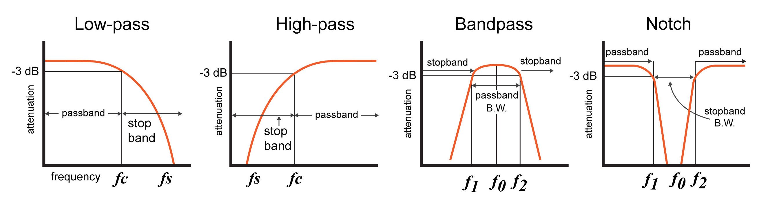
The response sketches provide a useful visual reference, but make one adjustment while studying them: physical filters have a transition region around their cutoff rather than a perfectly abrupt corner.

One cutoff frequency

Some responses have one side that is passed and one side that is attenuated. They therefore have one cutoff frequency, $f_c$, or equivalently ${\omega }_c$.

What the curve does as frequency increases	Passband	Stopband	Cutoff
Starts high and falls	Frequencies below the cutoff	Frequencies above the cutoff	One $-3\text{dB}$ crossing
Starts low and rises	Frequencies above the cutoff	Frequencies below the cutoff	One $-3\text{dB}$ crossing

For a falling curve with a $0\text{dB}$ passband plateau, find the horizontal level

$$-3.01\text{dB}$$

and locate its intersection with the curve. Project vertically down to the frequency axis. That frequency is $f_c$.

For a rising curve, use exactly the same method. The curve approaches its passband level from below, intersects the $3\text{dB}$-down line once, and continues toward the high-frequency passband.

Two cutoff frequencies

Other responses pass or reject a bounded range of frequencies. They have two $-3\text{dB}$ intersections:

$$f_{c1}$$

and

$$f_{c2}$$

where

$$f_{c1}<f_{c2}$$

Shape of response	Passband location	Stopband location	Cutoff frequencies
A central hump	Between $f_{c1}$ and $f_{c2}$	Below $f_{c1}$ and above $f_{c2}$	The two sides of the hump at $-3\text{dB}$ from its peak
A central dip or notch	Below $f_{c1}$ and above $f_{c2}$	Between $f_{c1}$ and $f_{c2}$	The two edges of the rejected interval, measured $3\text{dB}$ below the passband

Thus, the number of cutoff frequencies immediately tells you something structural:

• One cutoff separates a low-frequency region from a high-frequency region.
• Two cutoffs bound a finite frequency interval.

In later RLC lessons, the frequencies between two cutoffs will also let you determine bandwidth, center frequency, and quality factor.

---

A reliable graph-reading procedure

Use this method whenever you encounter a filter magnitude response, whether it is a smooth measured curve, a Bode plot, or a textbook sketch.

1. Read both axes and their units.
   Check whether frequency is labeled in $\text{Hz}$, $\text{kHz}$, $\text{MHz}$, or $\text{rad/s}$. Check whether the vertical scale is linear magnitude, gain in dB, or attenuation in dB.

2. Locate the intended maximum-response region.
   A flat plateau or the top of a resonant peak normally supplies the passband reference level $G_{\text{PB}}$.

3. Determine the half-power level.
   On a dB plot, mark:

   $$G_{\text{PB}}-3.01\text{dB}$$

   On a linear-magnitude plot, mark:

   $$\frac{|H{|}_{\text{PB}}}{\sqrt{2}}$$

4. Find every intersection of the response curve with that level.
   A one-sided response has one intersection. A bounded band has two.

5. Read the corresponding frequency or frequencies.
   These are the cutoff frequencies.

6. Identify passed and attenuated regions from the curve height.
   The region near the intended maximum is the passband. The region where the level is far lower is the stopband.

There is one practical caution. In a real design specification, the passband may be defined by a tolerance such as “no more than $1\text{dB}$ loss,” while the stopband may be defined by a requirement such as “at least $40\text{dB}$ attenuation.” The frequencies between those specified regions form a transition band.

At this introductory stage, the cutoff frequency is the conventional $-3\text{dB}$ marker that lets you summarize the response conveniently. It is not a claim that all frequencies just beyond cutoff are already strongly suppressed.

---

Worked plot interpretations

Example 1: A one-sided falling response

Suppose a graph has these features:

• The curve is essentially flat at $0\text{dB}$ from $10\text{Hz}$ to about $800\text{Hz}$.
• It crosses $-3\text{dB}$ at $1.0\text{kHz}$.
• It reaches $-20\text{dB}$ at $10\text{kHz}$.

The interpretation is:

$$f_c=1.0\text{kHz}$$

Frequencies well below $1.0\text{kHz}$ lie in the passband. Frequencies well above $1.0\text{kHz}$ lie in the attenuated region and eventually meet whatever stopband requirement is specified. The curve is falling with increasing frequency.

Notice that the point at $1.0\text{kHz}$ itself has neither full passband magnitude nor deep stopband attenuation:

$$|H(f_c)|=0.707|H{|}_{\text{PB}}$$

It is the standardized boundary marker.

Example 2: A central passed region

Suppose a response rises from very low levels, reaches a peak of $0\text{dB}$, then falls again. The curve crosses $-3\text{dB}$ at:

$$f_{c1}=9.6\text{kHz}$$

and

$$f_{c2}=10.4\text{kHz}$$

The frequency range that is passed with relatively little attenuation lies between the two cutoff frequencies:

$$9.6\text{kHz}\le f\le 10.4\text{kHz}$$

The regions below $9.6\text{kHz}$ and above $10.4\text{kHz}$ are attenuated.

The important habit is to identify the passband from the high portion of the curve, not from the fact that there happen to be two cutoff labels.

Example 3: A central rejected region

Now reverse the previous shape. Suppose the response remains close to $0\text{dB}$ at low and high frequencies but drops sharply around one frequency. The two $-3\text{dB}$ crossings occur at:

$$f_{c1}=49\text{Hz}$$

and

$$f_{c2}=51\text{Hz}$$

The interval between these cutoffs is attenuated:

$$49\text{Hz}\le f\le 51\text{Hz}$$

The low-frequency and high-frequency regions outside that interval are the passbands. Such a response is useful when one narrow interfering component, such as mains-related noise, must be rejected while frequencies on either side should remain available.

---

Avoid these common interpretation errors

Treating every cutoff as exactly $-3\text{dB}$ on the vertical scale.
It is $-3\text{dB}$ only when the passband reference is $0\text{dB}$. Otherwise, subtract $3.01\text{dB}$ from the actual passband level.

Confusing frequency with angular frequency.
A graph labeled $10^4\text{rad/s}$ does not show $10\text{kHz}$. Convert when necessary:

$$f=\frac{\omega }{2\pi }$$

Calling a frequency at the bottom of a notch a cutoff.
The deep minimum identifies the most strongly rejected frequency. The cutoffs are the two points where the response has risen to the $-3\text{dB}$ level relative to the passband.

Assuming cutoff means zero output beyond that point.
Passive analog filters roll off gradually. Cutoff means a defined attenuation level, not complete removal of all other frequencies.

Ignoring a logarithmic frequency axis.
On a Bode plot, equal horizontal distances often represent equal frequency ratios, not equal frequency differences. Read the tick labels rather than estimating as though the axis were linear.

---

Key takeaways

A magnitude response shows output level as a function of frequency. To interpret it:

• The passband is the region with little attenuation relative to the intended maximum response.
• The stopband is the region with substantial attenuation.
• A cutoff occurs where the magnitude has dropped to:

$$\frac{1}{\sqrt{2}}$$

of the passband magnitude, or where gain is:

$$3.01\text{dB}$$

below the passband reference.

• A one-sided response has one cutoff frequency; a response that passes or rejects a bounded interval has two cutoff frequencies.
• Real filters transition gradually, so cutoff is a conventional and useful reference point rather than an abrupt physical boundary.

Next, you will use these visual signatures to formally classify ideal magnitude responses as low-pass, high-pass, bandpass, or bandreject filters.