Maxwell's Equations and Electromagnetic Wave Propagation

Hello! Welcome to the final lesson in our module on Maxwell's equations.

In our last session, we explored the two dynamic laws: Faraday's Law, where a changing magnetic field creates an electric field, and the Ampère-Maxwell Law, where currents and changing electric fields create a magnetic field. We noted the beautiful symmetry between these two laws and concluded with a teaser: this interplay is the very origin of light.

Today, we will see that prediction come to life. Our learning outcome is to describe how the interplay between changing electric and magnetic fields, as described by Maxwell's equations, leads to the propagation of electromagnetic waves. We will connect the conceptual "dance" of the fields to the mathematical formalism and see how Maxwell was able to predict the speed of light from first principles.

The Perpetual Dance of Electric and Magnetic Fields

The previous lesson established a feedback loop:

1. A changing magnetic field ($\frac{d\vec{B}}{dt}$) induces a circulating electric field ($\vec{E}$). (Faraday's Law)
2. A changing electric field ($\frac{d\vec{E}}{dt}$) induces a circulating magnetic field ($\vec{B}$). (Ampère-Maxwell Law)

Imagine initiating a disturbance—for example, by accelerating a charge. This creates a changing electric field in the space around it. According to the Ampère-Maxwell law, this changing $\vec{E}$ field must generate a changing, circulating $\vec{B}$ field. But this new $\vec{B}$ field is itself changing, so by Faraday's law, it must generate a new changing, circulating $\vec{E}$ field a little further out.

This process continues, with each field generating the other in a self-sustaining "leapfrog" effect, propagating outward through space. This propagating disturbance is an electromagnetic wave.

To see this dynamic process in action, let's watch a segment from a CrashCourse video that illustrates it using a practical example: an antenna.

The video highlights two crucial properties of these waves:

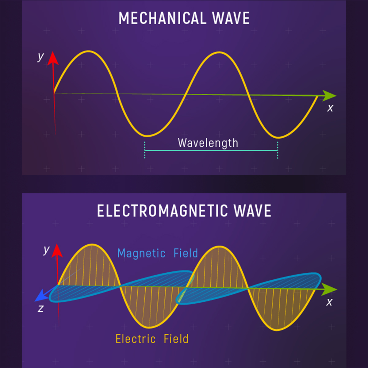
• The electric field ($\vec{E}$), the magnetic field ($\vec{B}$), and the direction of propagation are all mutually perpendicular.
• The wave is transverse, meaning the oscillations of the fields are perpendicular to the direction the wave is traveling.

This structure is a direct consequence of the "circulating" or "curling" nature of the induced fields described by the curl operator in the differential forms of Faraday's and Ampère-Maxwell's laws.

From Maxwell's Equations to the Wave Equation

This conceptual picture has a firm mathematical foundation. By combining the two dynamic laws in their differential (curl) forms, we can derive a famous partial differential equation that governs wave motion.

The following reading walks through the unification of the electric and magnetic fields and shows how the wave equation emerges directly from Maxwell's equations in a vacuum (a region with no charges or currents).

The derivation you just saw is one of the pinnacles of 19th-century physics. It demonstrates that the existence of waves is not an add-on to the theory, but a direct and necessary consequence of the laws of electricity and magnetism. The term that falls out of the derivation, $1/{\mu }_0{ϵ}_0$, represents the square of the wave's propagation speed.

A Physical Derivation of the Wave's Speed

Maxwell calculated this speed using the values of ${\mu }_0$ (the permeability of free space, from experiments with magnetic forces) and ${ϵ}_0$ (the permittivity of free space, from experiments with electric forces). The result was approximately $3\times 10^8$ m/s, the known speed of light. This was overwhelming evidence that light is an electromagnetic wave.

Let's explore a beautiful physical argument that derives this speed without resorting to the differential wave equation. It uses only the integral forms of Faraday's and Ampère-Maxwell's laws and a simple thought experiment.

The setup is a large, flat sheet of current that is suddenly switched on. We want to find out how fast the resulting magnetic and electric fields propagate outwards from the sheet.

Let's recap the elegant logic of that derivation:

1. The Setup: A current sheet is switched on at $t=0$. We assume the $\vec{B}$ field and an accompanying $\vec{E}$ field propagate outwards at some unknown speed $v$.
2. Ampère-Maxwell Law: Applying $\oint \vec{B}\cdot d\vec{l}={\mu }_0(I_{enc}+{ϵ}_{0}d{\Phi }_E/dt)$ to a rectangular loop that extends beyond the wave front, the left side is zero. For the right side to also be zero, the changing electric flux must exactly cancel the conduction current. This gives a relationship between $E$, $v$, and the current per unit length $I$. Combining this with the known static field $B={\mu }_{0}I/2$, we find $B={\mu }_0{ϵ}_{0}vE$.
3. Faraday's Law: Applying $\oint \vec{E}\cdot d\vec{l}=-d{\Phi }_B/dt$ to a different rectangular loop whose area is swept by the propagating $\vec{B}$ field gives a second, simpler relationship: $E=vB$.
4. The Conclusion: We have a system of two linear equations for $E$ and $B$. The only way for a non-trivial solution to exist is if the constants satisfy a specific relationship. Substituting $E=vB$ into the first equation gives $B={\mu }_0{ϵ}_{0}v(vB)$, which simplifies to $1={\mu }_0{ϵ}_0{v}^2$, or $v=1/\sqrt{{\mu }_0{ϵ}_0}$.

This physical argument powerfully demonstrates that the speed of light is not an arbitrary number but is baked into the very fabric of electric and magnetic interactions.

Conclusion

In this lesson, we have seen how the symmetric, dynamic interplay between electric and magnetic fields leads to one of the most profound predictions in physics: the existence of self-propagating electromagnetic waves.

Key Takeaways:

• The feedback loop between Faraday's Law (changing $\vec{B}$ $\to$ $\vec{E}$) and the Ampère-Maxwell Law (changing $\vec{E}$ $\to$ $\vec{B}$) creates a self-sustaining wave.
• Electromagnetic waves are transverse, with the electric field, magnetic field, and direction of propagation being mutually perpendicular.
• Combining Maxwell's equations mathematically leads to the wave equation, confirming that these waves are a necessary consequence of the theory.
• The speed of these waves in a vacuum is determined solely by the fundamental constants of electricity and magnetism, ${\mu }_0$ and ${ϵ}_0$, and is equal to the speed of light, $c$.

This concludes our module on the theoretical foundations of electromagnetism. You now have a complete picture, from the static sources of fields in Gauss's laws to the dynamic interplay that gives rise to light itself.

Preview of the Next Module:
We will now shift our focus to the practical application of these principles in the context of AC Circuits and Power. Our first lesson will introduce the sinusoidal functions used to describe alternating current and voltage and distinguish between peak and RMS (root mean square) values, which are essential for analyzing the behavior of circuits in our homes and power grids.