Quantum Phase Estimation Algorithm

Hello! Welcome to the next lesson in our exploration of foundational quantum algorithms.

In our previous lesson, we analyzed the gate complexity of the Quantum Fourier Transform (QFT). We established its $O(n^2)$ complexity, which translates to an exponential speedup over the classical Fast Fourier Transform's $O(N\log N)$ for a state space of size $N=2^n$. We also noted that the QFT's power is unlocked in algorithms where we can extract specific global properties from the transformed state without needing to measure all the amplitudes.

Today, we will study the canonical application that does exactly this: the Quantum Phase Estimation (QPE) algorithm. This powerful algorithm serves as a core subroutine in many other quantum algorithms, most famously in Shor's algorithm for factoring. Our goal is to implement the quantum phase estimation algorithm to find the phase of an eigenvalue of a unitary operator.

We will build the algorithm from the ground up, see how it leverages the Inverse QFT, implement it in code, and analyze its performance.

1. The Phase Estimation Problem

First, let's formally define the problem we want to solve. We are given a unitary operator $U$ and one of its eigenvectors $|\psi ⟩$. By definition, they satisfy the eigenvalue equation:

$$U|\psi ⟩=\lambda |\psi ⟩$$

Since $U$ is unitary, its eigenvalues must be complex numbers with a magnitude of 1. We can therefore write any eigenvalue $\lambda$ in the form $\lambda =e^{2\pi i\varphi }$, where $\varphi \in [0,1)$ is the phase. The goal of the Quantum Phase Estimation algorithm is to find a good approximation of this phase $\varphi$.

The following video provides an excellent and precise definition of the problem.

{
    "intro": "This video from the Qiskit YouTube channel clearly sets up the phase estimation problem, explaining the inputs, the promise, and the goal.",
    "resource_id": "cbbc4",
    "relevant_parts": [0],
    "instructions": "Please watch from 05:43 to 11:56. Pay close attention to how the phase \(\phi\) is parameterized and what it means to find an 'm-bit approximation' to it.",
    "estimated_time": "6 minutes"
}

As the video highlights, QPE is typically a subroutine within a larger algorithm. We are given a circuit that implements $U$ and a way to prepare the state $|\psi ⟩$, and our task is to compute $\varphi$.

2. The Core Mechanism: Phase Kickback

The physical mechanism that makes QPE possible is phase kickback, a phenomenon you've encountered before in algorithms like Deutsch-Jozsa. We can gain intuition for the full algorithm by first examining a simple circuit that uses one auxiliary qubit (often called a control or counting qubit) to learn something about $\varphi$.

This "warmup" exercise demonstrates how the eigenvalue's phase is imprinted onto the state of the auxiliary qubit.

{
    "intro": "The next segment of the same video walks through a simple single-qubit version of phase estimation.",
    "resource_id": "cbbc4",
    "relevant_parts": [1],
    "instructions": "Please watch from 11:56 to 17:17. Focus on how the controlled-U operation leads to the state \(\frac{1}{\sqrt{2}}(|0\rangle + e^{2\pi i \phi} |1\rangle)\) in the control qubit, and how the final Hadamard gate transforms this into a state whose measurement probabilities depend on \(\cos^2(\pi\phi)\) and \(\sin^2(\pi\phi)\).",
    "estimated_time": "5 minutes"
}

This simple procedure gives us some information about $\varphi$, but it's imprecise and ambiguous (e.g., it cannot distinguish between $\varphi$ and $1-\varphi$). To do better, we need more precision.

3. From a Single Bit to High Precision

To improve the precision of our estimate, we need to add more counting qubits. The key idea is to use each counting qubit to control successively higher powers of the unitary, $U,U^2,U^4,\dots ,U^{2^{m-1}}$.

Let's see how this works. If we have a circuit for a controlled-$U$ operation, applying it $k$ times is equivalent to a controlled-$U^k$ operation. Since $|\psi ⟩$ is an eigenvector of $U$ with eigenvalue $e^{2\pi i\varphi }$, it is also an eigenvector of $U^k$ with eigenvalue $(e^{2\pi i\varphi }{)}^k=e^{2\pi ik\varphi }$.

The full QPE algorithm uses this fact with $m$ counting qubits.

1. Each of the $m$ counting qubits is put into a $|+⟩$ state using a Hadamard gate.
2. The $k$-th counting qubit is used to control the application of $U^{2^{k-1}}$ to the $|\psi ⟩$ register.
3. Through phase kickback, the state of the counting register becomes a superposition where each basis state $|j⟩$ has acquired a phase related to $j\cdot \varphi$.
4. This resulting state has exactly the form of a Quantum Fourier Transform of the phase we want to find. Therefore, applying an Inverse Quantum Fourier Transform (IQFT) to the counting register will rotate it back to a computational basis state that encodes the bits of $\varphi$.

The following video provides a brilliant step-by-step construction of this idea, building from two qubits to the general case.

4. The General Algorithm and its Implementation

We are now ready to look at the complete QPE algorithm and its implementation. The circuit diagram below summarizes the structure we just derived.

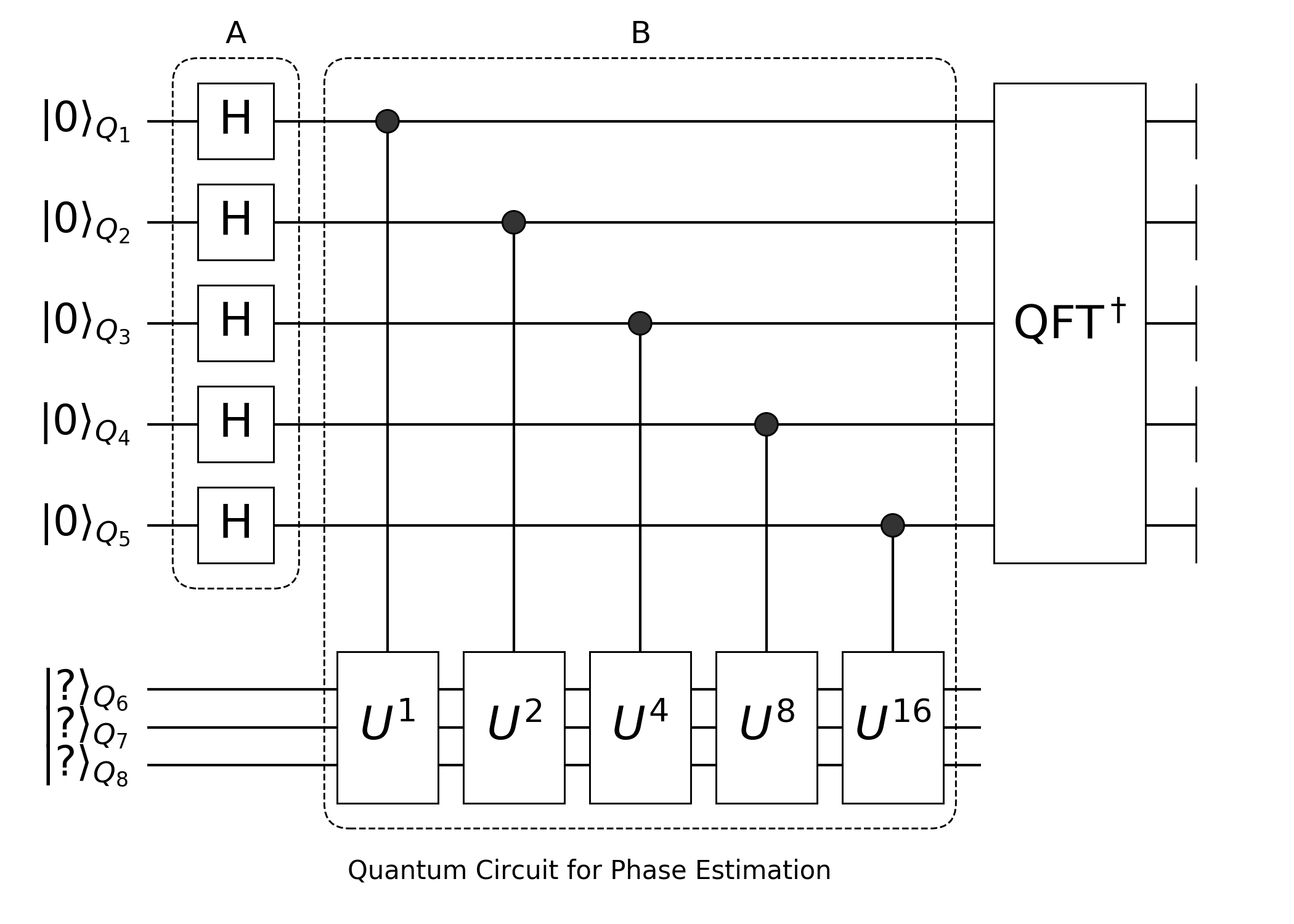
The state of the $m$ counting qubits just before the IQFT is:

$$\frac{1}{2^{m/2}}\sum _{k=0}^{2^m-1}{e}^{2\pi i\varphi k}|k⟩$$

This is precisely the quantum Fourier transform of a state that is sharply peaked at the value $2^m\varphi$. Applying the IQFT thus yields the state $|2^m\varphi ⟩$, which upon measurement gives us the $m$-bit binary representation of the phase $\varphi$.

The following reading provides a concise mathematical derivation and a Qiskit code snippet for implementing this.

Practical Implementation

Let's solidify this by implementing the algorithm for a concrete example. We will find the phase of a T-gate, which is a phase gate $P(\pi /4)$.

• Unitary $U$: T-gate, with matrix $\left(\begin{array}{cc}1& 0\\ 0& e^{i\pi /4}\end{array}\right)$.
• Eigenvector $|\psi ⟩$: $|1⟩$.
• Eigenvalue Equation: $T|1⟩=e^{i\pi /4}|1⟩$.

Here, the eigenvalue is $\lambda =e^{i\pi /4}$. Comparing this to the standard form $e^{2\pi i\varphi }$, we have $2\pi \varphi =\pi /4$, which means the phase is $\varphi =1/8=0.125$.

In binary, $\varphi =0.001_2$. To estimate this phase, we need at least 3 counting qubits. If we use $m=3$ counting qubits, we expect the measurement of the counting register to yield the binary string 001, which corresponds to the integer 1. The estimated phase would then be $\frac{1}{2^3}=\frac{1}{8}$.

Below is a complete Qiskit implementation.

import numpy as np
from qiskit import QuantumCircuit, transpile, assemble, Aer
from qiskit.visualization import plot_histogram
from qiskit.circuit.library import QFT

# --- Parameters ---
# Number of counting qubits determines the precision of the phase estimation
m = 3  # We need 3 qubits to represent 1/8
# Number of qubits for the eigenstate
n = 1

# --- The Unitary Operator and its controlled version ---
# We want to find the phase of a T-gate
# T|1> = exp(i*pi/4)|1>, so phi = 1/8
def controlled_t_power(power):
    """Returns a controlled T-gate raised to a power."""
    qc = QuantumCircuit(2)
    angle = (np.pi / 4) * power
    qc.cp(angle, 0, 1) # cp is the controlled-phase gate
    return qc.to_gate(label=f"c-T^{power}")

# --- Build the QPE Circuit ---
# Create a circuit with m counting qubits and n eigenstate qubits
qpe = QuantumCircuit(m + n, m)

# 1. Prepare the eigenstate |1> in the target register
qpe.x(m) # Target qubit is at index m
qpe.barrier()

# 2. Apply Hadamard gates to the counting qubits
for qubit in range(m):
    qpe.h(qubit)

# 3. Apply the controlled unitary operations
for i in range(m):
    power = 2**i
    # Control qubit is i, target qubit is m
    qpe.cp((np.pi/4)*power, i, m)

qpe.barrier()

# 4. Apply the inverse QFT
# Note: Qiskit's QFT is ordered from most to least significant bit,
# which matches our circuit construction.
iqft_gate = QFT(num_qubits=m, inverse=True).to_gate()
qpe.append(iqft_gate, range(m))

qpe.barrier()

# 5. Measure the counting qubits
qpe.measure(range(m), range(m))

# Display the circuit
print("Quantum Phase Estimation Circuit:")
print(qpe)

# --- Simulation ---
simulator = Aer.get_backend('qasm_simulator')
t_qpe = transpile(qpe, simulator)
qobj = assemble(t_qpe)
results = simulator.run(qobj, shots=2048).result()
counts = results.get_counts()

# --- Interpretation ---
# The measured bitstring is reversed in Qiskit, so we reverse it back
measured_int = int(list(counts.keys())[0], 2)
estimated_phi = measured_int / (2**m)

print(f"\nSimulation Results: {counts}")
print(f"Most frequent measurement: {list(counts.keys())[0]}")
print(f"Corresponds to integer: {measured_int}")
print(f"Estimated phase (phi): {estimated_phi}")
print(f"True phase (phi): {1/8}")

plot_histogram(counts)

When you run this code, you will see that the measurement result is 001 with probability 1. This is because the phase $\varphi =1/8$ can be represented exactly with 3 bits.

5. Accuracy and Computational Cost

What happens if the phase cannot be represented exactly with $m$ bits? In this case, the IQFT produces a superposition of states, but the measurement outcomes will be peaked around the true value.

A formal analysis shows that the probability of measuring the best $m$-bit approximation to $\varphi$ is at least $4/{\pi }^2\approx 40.5\%$. This is a remarkable result: even with a single run, we have a high chance of getting the best possible answer for the given number of counting qubits. By repeating the algorithm a few times, we can determine the correct phase with very high confidence.

As the video points out, the main bottleneck of QPE is the implementation of the controlled-$U^{2^k}$ operations for large $k$. If the circuit for $U$ has $G$ gates, a naive implementation of $U^{2^{m-1}}$ would require $O(G\cdot 2^m)$ gates, an exponential cost that would negate any quantum advantage. Fortunately, for specific problems like the period-finding at the heart of Shor's algorithm, there are efficient classical methods to compute the circuit for modular exponentiation, which allows us to construct the required controlled unitaries efficiently.

Conclusion

In this lesson, we have constructed and implemented the Quantum Phase Estimation algorithm, a cornerstone of quantum computing.

Key Takeaways:

• Purpose: QPE estimates the phase $\varphi$ of an eigenvalue $e^{2\pi i\varphi }$ of a unitary operator $U$.
• Mechanism: It uses phase kickback to transfer phase information from an eigenstate $|\psi ⟩$ to a register of $m$ counting qubits.
• Core Components: The algorithm involves initializing the counting qubits with Hadamard gates, applying a series of controlled-$U^{2^k}$ operations, and finally using an Inverse QFT to transform the phase information into a measurable computational basis state.
• Precision and Success: The precision of the estimate is determined by the number of counting qubits, $m$. For a phase that cannot be exactly represented, the algorithm still provides the best $m$-bit approximation with a probability of at least ~40%.
• Cost: The main computational cost lies in implementing the controlled-$U^{2^k}$ gates for large $k$, which can be prohibitive unless an efficient construction for these circuits is known.

We now have the central tool needed to tackle Shor's algorithm. In our next lesson, we will see how the problem of factoring a large number can be reduced to finding the period of a specific function. We will then be ready to use QPE to solve that period-finding problem, unlocking the power of quantum computation for cryptography.