Building the Period-Finding Circuit with QPE and Modular Exponentiation

Hello! Welcome back to our deep dive into foundational quantum algorithms.

In our last lesson, we constructed the reversible quantum circuit for modular exponentiation, $U_{a, N} : ∣ x ⟩ ∣1 ⟩ \mapsto ∣ x ⟩ ∣ a^{x} (mod N)⟩$ . This circuit, based on the classical repeated squaring algorithm, is the computational engine at the heart of Shor's algorithm.

Today, we will integrate this engine into a larger framework to achieve our goal: finding the period $r$ of $a$ modulo $N$ . Our learning outcome is to integrate the modular exponentiation oracle into the Quantum Phase Estimation framework to construct the complete circuit for the period-finding subroutine. This lesson will connect all the pieces—the number theory, the quantum circuit design, and the Quantum Fourier Transform—into a single, powerful quantum procedure.

1. The Quantum Phase Estimation (QPE) Algorithm

The core quantum primitive we will use is Quantum Phase Estimation (QPE). Its purpose is to determine the eigenvalue of a unitary operator.

The problem is as follows: Given a unitary operator $U$ and one of its eigenvectors $∣ ψ ⟩$ such that $U ∣ ψ ⟩ = e^{2 πi ϕ} ∣ ψ ⟩$ , the goal is to find the phase $ϕ$ .

The QPE algorithm uses two quantum registers:

A counting register of $t$ qubits, initialized to $∣0 ⟩^{\otimes t}$ . The number of qubits $t$ determines the precision of our phase estimate.
A state register of $n$ qubits, which holds the eigenvector $∣ ψ ⟩$ .

The general procedure is a beautiful application of phase kickback and the Quantum Fourier Transform. The following video provides a detailed and clear explanation of the QPE algorithm.

Phase Estimation and Factoring | Understanding Quantum Information & Computation | Lesson 07

Let's begin with a thorough review of the Quantum Phase Estimation (QPE) algorithm. This video from the Qiskit YouTube channel provides an excellent walkthrough, starting from the basic problem definition and building up to the general procedure.

Please watch the following segments: 'Phase Estimation Problem Definition and Warm-up' (05:43 - 17:17) to understand the core problem. 'Generalizing Phase Estimation with Multiple Control Qubits and QFT' (17:17 - 32:21) to see how precision is increased. 'Generalized Phase Estimation Procedure and Cost Analysis' (41:45 - 48:22) for the complete, general algorithm. Focus on the structure of the circuit: the two registers, the sequence of controlled-U powers, and the crucial role of the inverse Quantum Fourier Transform (QFT⁻¹).

2. Applying QPE to the Order-Finding Problem

Now, let's specialize this general QPE framework for our specific task of finding the order $r$ . This requires us to define the unitary operator $U$ , its eigenvectors, and the initial state we will use.

The Unitary Operator

The unitary operator whose eigenvalues encode the period $r$ is not the full modular exponentiation circuit from last lesson, but rather the simpler modular multiplication operator:

U_{a} ∣ y ⟩ = ∣ (a \cdot y) (mod N)⟩

where $y$ is an integer with $0 \leq y < N$ and $gcd (a, N) = 1$ . This operator is unitary because it simply permutes the basis states $∣0 ⟩, ∣1 ⟩, \dots, ∣ N - 1 ⟩$ .

Eigenstates and Eigenvalues

The eigenstates of this operator are Fourier-type states. For integers $s$ where $0 \leq s < r$ , the states are defined as:

∣ u_{s} ⟩ = \frac{1}{r} k = 0 \sum r - 1 e^{- 2 πi s k / r} ∣ a^{k} (mod N)⟩

Applying our unitary $U_{a}$ to such a state reveals its eigenvalue:

U_{a} ∣ u_{s} ⟩ = U_{a} (\frac{1}{r} k = 0 \sum r - 1 e^{- 2 πi s k / r} ∣ a^{k} (mod N)⟩) = e^{2 πi s / r} ∣ u_{s} ⟩

The phase of the eigenvalue is $ϕ_{s} = s / r$ . This is exactly what we need! If we can estimate these phases, we can find the period $r$ .

Preparing the Input State

A challenge arises here: to prepare an eigenstate $∣ u_{s} ⟩$ , we need to know $r$ , which is the very quantity we are trying to find. The solution is a remarkably elegant trick. Instead of preparing a single eigenstate, we prepare a state that is an equal superposition of all of them. As it turns out, the simple state $∣1 ⟩$ is exactly this superposition:

∣1 ⟩ = \frac{1}{r} s = 0 \sum r - 1 ∣ u_{s} ⟩

The following reading from your alma mater's lecture notes provides a concise derivation of these facts.

Quantum Computing (CST Part II) - Lecture 10

Let's formalize the connection between QPE and order-finding. These lecture notes from the University of Cambridge CST Part II course provide a rigorous mapping.

Please read the following sections: 'Order finding using quantum phase estimation' (page 7): This defines the specific unitary operator U whose eigenvalues encode the period. 'The eigenvalues of U' and 'A superposition of eigenstates of U' (pages 11-12): These sections derive the eigenstates and eigenvalues of U, and crucially, show why the simple state |1⟩ is the correct input for the state register. Pay close attention to the form of the eigenvalues, e^{2πis/r}, as this is the phase we aim to estimate.

By using $∣1 ⟩$ as the input to the state register, the linearity of quantum mechanics ensures that the QPE circuit will simultaneously estimate the phase for each eigenstate in the superposition. A measurement of the counting register will then yield an estimate for $s / r$ for a randomly chosen $s$ .

3. Constructing the Complete Period-Finding Circuit

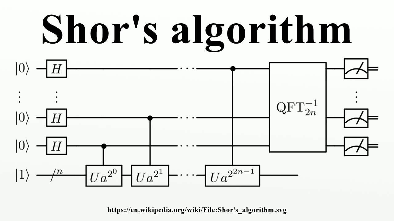
We are now ready to assemble the full circuit. The QPE algorithm requires us to implement a sequence of controlled unitaries: C- $U_{a}$ , C- $U_{a}^{2}$ , C- $U_{a}^{4}$ , ..., C- $U_{a}^{2^{t - 1}}$ .

This is precisely where the modular exponentiation circuit from our previous lesson comes into play. Note that $U_{a}^{k} ∣ y ⟩ = ∣ (a^{k} y) (mod N)⟩$ . This is just modular multiplication by the constant $a^{k}$ .

The "trick" is that instead of applying the $U_{a}$ gate $2^{j}$ times, we can classically compute $c_{j} = a^{2^{j}} (mod N)$ (using exponentiation by squaring) and then implement a single controlled-multiplication by $c_{j}$ . This is exponentially faster.

The modular exponentiation circuit we built last lesson, which maps $∣ x ⟩ ∣1 ⟩ \to ∣ x ⟩ ∣ a^{x} (mod N)⟩$ , is exactly the implementation of this entire sequence of controlled operations, where the qubits of $∣ x ⟩$ are the control qubits for QPE.

This is the central point of integration.

Quantum Computing (CST Part II) - Lecture 10

The QPE algorithm requires a series of controlled gates: C-U, C-U², C-U⁴, and so on. A naive implementation would be exponentially costly. This is the key integration point with our previous lesson.

Please read 'Implementing the series of controlled-U^2j gates' and 'Complexity of implementing the controlled-U^2j gates' (pages 9-10). This section explicitly details how classical pre-computation of a^{2^j} mod N allows for an efficient construction of the required controlled unitaries. This is the 'modular exponentiation oracle' in action.

The complete circuit for the period-finding subroutine is therefore a direct implementation of QPE tailored for this problem.

Caption: The complete quantum circuit for the period-finding subroutine. The top $t$-qubit register is the counting register, and the bottom $n$-qubit register is the state register. The circuit integrates the key components: (1) Hadamard gates to create a superposition in the counting register, (2) a series of controlled modular multiplication gates (U_a, U_a^2, etc.) which constitute the modular exponentiation oracle, and (3) an inverse Quantum Fourier Transform (QFT⁻¹) to extract the phase information into a measurable state. The state register is initialized to |1⟩, which acts as a superposition of the required eigenstates.

4. From Phase to Period: Classical Post-Processing

After running the circuit and measuring the $t$ -qubit counting register, we obtain a measurement result, an integer $m$ . This gives us the approximation:

\frac{m}{2 ^{t}} \approx \frac{s}{r}

for some random $s \in {0, \dots, r - 1}$ .

Our final task is to recover $r$ from this approximation. This is a classic problem in number theory that can be solved efficiently using the continued fractions algorithm. This algorithm takes a real number (our $m / 2^{t}$ ) and finds the "best" rational approximation with a denominator below a certain bound.

If we choose $t$ large enough (typically $t \approx 2 lo g_{2} N$ ), the approximation $m / 2^{t}$ will be close enough to $s / r$ for the continued fractions algorithm to recover the fraction $s / r$ exactly (in lowest terms).

The denominator of the resulting fraction is our candidate for the period $r$ . If $gcd (s, r) \neq = 1$ , the denominator will be a factor of $r$ . By repeating the entire quantum procedure a few times and taking the least common multiple of the resulting denominators, we can determine $r$ with very high probability.

The final part of the Qiskit video explains this post-processing step.

Phase Estimation and Factoring | Understanding Quantum Information & Computation | Lesson 07

After measuring the counting register, we get an integer that gives us a binary approximation of a fraction s/r. To recover the period r, we need a classical algorithm to find this fraction. The Qiskit video explains this final step.

Please watch the segment from 57:50 to 1:04:40 within the 'Order Finding Problem and Connection to Phase Estimation' part. This section explains how the measurement result is used with the continued fraction algorithm to find the period r, even when we only get s/r for a random s.

Conclusion

We have now assembled the complete quantum subroutine for period-finding, the core of Shor's algorithm.

Key Takeaways:

The period-finding algorithm is a specific application of the Quantum Phase Estimation (QPE) framework.
The relevant unitary is the modular multiplication operator $U_{a} ∣ y ⟩ = ∣ (a y) (mod N)⟩$ , whose eigenvalues $e^{2 πi s / r}$ encode the period $r$ .
The required input eigenstate is prepared by using the simple state $∣1 ⟩$ , which is an equal superposition of all the necessary eigenstates.
The sequence of controlled unitaries (C- $U_{a}^{2^{j}}$ ) required by QPE is implemented efficiently by the modular exponentiation circuit we constructed in the previous lesson. This is the "oracle".
The final measurement from QPE gives an estimate of the phase $s / r$ , which is then processed by the classical continued fractions algorithm to find the period $r$ .

In our next lesson, we will analyze the computational complexity of this entire procedure, comparing it to the best classical factoring algorithms like the General Number Field Sieve, to fully appreciate the source and magnitude of the quantum speedup.